Introduction

Regression Discontinuity is a non-experimental research design for analyzing causal effects. The most important feature of this design is that the probability of receiving a treatment changes drastically at a known threshold.

In a Sharp RDD, the probability of receiving the treatment jumps discretely at a particular threshold value of the assignment variable. In other words, if X is below the cutoff (C), there’s a 0 probability of receiving treatment. If X is equal to or larger than C, the probability of receiving treatment is 1. In this case, compliance is perfect: everyone gets the treatment or control condition they’re assigned to.

However, in a Fuzzy RDD, the treatment’s probability changes discontinuously at the cutoff but does not jump immediately from zero to one. ​The treatment now has the property of imperfect compliance. This means that some units with a score higher than the cutoff fail to receive the treatment or some units with a score lower than the cutoff receive the treatment.

In both designs, treatment assignment is determined by whether the assignment variable X is greater than or equal to the cutoff C, denoted mathematically as $T_{i} = \mathbb{1}(X_{i} >= c)$. While the treatment assignment rule remains the same in Fuzzy RD, the shift in treatment probability at the cutoff is less extreme compared to Sharp RD.

Fuzzy RD Assumptions

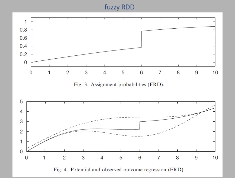
Figure 3 in Imbens and Lemieux (2008) illustrates the conditional probability of receiving the treatment for a Fuzzy RD. Like in Sharp RD, there is a jump at $D_{i}(1)$, but it’s smaller than 1. The following graph displays expected potential outcomes, marked by dashed lines, based on the treatment covariate $X_{i}$ indicated by dashed lines. The solid line represents observed outcomes, which is a weighted average calculated using assignment probabilities of the figure on top. The upper and lower dashed lines depict potential outcomes if all or no units were treated, respectively. The solid line shows observed outcomes, revealing a distinct jump at the cutoff.

The graph leads us to three core assumptions for Fuzzy RDD:

1. Expectations of potential outcomes are smooth at the cutoff (Continuity Assumption):
   Evidenced by the continuous dashed lines around the cutoff of 6.
2. There is a discontinuity in treatment probability:
   Highlighted by the jump at the cutoff in the solid line, indicating that while it’s not a 0-1 switch like in Sharp RDD, a discontinuity still occurs.
3. $E[Y_{0,1}|X_{i} = c]$ and $E[Y_{1,i}|X_{i} = c]$ do not depend on $D_{i}$ (Monotonicity).
   This is essential to eliminate local selection bias, ensuring that units near the cutoff cannot intentionally be just above or below it, making the treatment assignment effectively random.

Continuity Assumption

The validity of a Sharp RD design relies on the continuity assumption, which means that the two potential outcomes are expected to be continuous at the threshold. In other words, in the absence of the treatment, the outcome would follow a smooth, continuous function across the cutoff (note that the dashed lines in the figure are smooth around the cutoff). This assumption ensures that the only ‘discontinuity’ or ‘jump’ in the outcomes around the cutoff is due to the treatment effect, enabling causal inference. Note, that this cannot be tested, and relies on the institutional background.

Fuzzy RD, similar to Sharp RD, also relies on the continuity assumption. However, due to imperfect compliance, there is a chance of treatment instead of a switch of turning treatment on, as is the case with perfect compliance. In a Fuzzy RD, this assumption must account for the fact that treatment assignment is probabilistic, not certain. This results in the estimated treatment effect in Fuzzy RD being a more localized (LATE) one, suitable for those who comply with the treatment they’re assigned around the threshold.

Assigned Treatment vs. Received Treatment

Since the treatment assigned is not always the same as the actual treatment received, we need different notations to distinguish between them. If the treatment assignment is noted with $T_{i}$, we define the treatment received with $D_{i}$, also known as treatment take-up. Therefore the main characteristic of Fuzzy RDD is that there are some units for which $T_{i} \neq D_{i}$.

$D_{i}$ has two values:

• $D_{i}(1)$: treatment received by $i$ when it is assigned to the treatment condition
• $D_{i}(0)$: treatment received by $i$ when it is assigned to the control condition

For instance, if unit $i$ receives treatment when assigned to the control condition, we then have $D_{i}(0) = 1$.

Estimation and Inference Methods

Non-compliance with treatment could occur because some units may decide to take or refuse the treatment, which introduces confounding between potential outcomes and compliance decisions. This can affect learning causal treatment effects for all units, in the absence of additional assumptions. Therefore, we need additional parameters, besides the average treatment effect, that can help with cases of non-compliance.

By applying the Sharp RD estimation strategy to the observed outcome in a Fuzzy RDD we estimate two parameters: $\tau_{Y}$ and $\theta_{Y}$.

$\tau_{Y}$ is estimated by comparing the average outcome of observations just below the cutoff to the average outcome of observations just above the cutoff, then by taking the limit of the two averages as the score approaches the cutoff.

$\theta_{Y}$ is obtained by applying a local randomization approach that compares observations in a small window $W$.

There are two strategies using these parameters:

• Focus on assumptions that allow for the interpretation of $\tau_{Y}$ and $\theta_{Y}$ as the effect of assigning the treatment on the outcome: Intention-To-Treat
• Focus on assumptions that allow learning about the effect of receiving the treatment on the outcome: Local Average Treatment Effect

Intention-to-treat Effects

The focus of the first strategy is to learn about the effects of the treatment assignment. The effects of assigning the treatment on any outcome are called intention-to-treat effects (ITT). There are two assumptions/approaches that can help obtain the ITT parameters: the continuity-based approach and the local randomization approach. After applying the two, the ITT parameters become:

• $\tau_{Y} = \mathbb{E}[Y_{i}(1) - Y_{i}(0) | X_{i} = c]$
• \(\theta_{Y} = \mathbb{E}_{W}[Y_{i}(1) - Y_{i}(0) | X_{i} \in W]\)

As for the second strategy, the focus is on studying the effects of receiving the treatment. The same two parameters are defined, but the outcome variable is now $D$ instead of $Y$. Therefore, the parameters become:

• $\tau_{D} = \mathbb{E}[D_{i}(1) - D_{i}(0) | X_{i} = c]$
• \(\theta_{D} = \mathbb{E}_{W}[D_{i}(1) - D_{i}(0) | X_{i} \in W]\)

Treatment Effects for Subpopulations

If the goal is to study the effect of the treatment received, the focus is then on the Fuzzy RD parameters:

• $\tau_{FRD} = \tau_{Y}/\tau_{D}$
• $\theta_{FRD} = \theta_{Y}/\theta_{D}$

We can define four groups of units according to the compliance decisions:

• compliers: units whose treatments received coincide with their treatment assigned
• never-takers: units who always refuse the treatment regardless of their assignment
• always-takers: units who always take the treatment no matter their assignment
• defiers: units who receive the other treatment than the one they are assigned

In a Sharp RDD, the average treatment effect can be estimated for a subpopulation whose running variable falls within a narrow range around the cutoff, technically, this can be made arbitrarily small. In contrast, a Fuzzy RDD requires the additional monotonicity assumption, previously discussed, to estimate the Local Average Treatment Effect (LATE) for a subpopulation with a forcing variable equal to the cutoff. Monotonicity is the assumption that there are no defiers inside $W$ or at or around the cutoff.

Bandwidth and Window Selection

The procedure for selecting bandwidth and window selection for the ITT parameters aligns with what is outlined in the Sharp RDD building block. However, when calculating $\tau_{FRD}$, which is a ratio, the question arises whether to use the same bandwidth for both the numerator and the denominator. If the focus is on the ITT effects ($\tau_{Y}$), then it is advisable to have different bandwidths for the denominator and numerator. On the other hand, if the focus is on the ratio $\tau_{FRD}$, then maintaining identical bandwidths enhances the transparency of the analysis.

See also

• A Practical Introduction to Regression Discontinuity Designs: Extensions - Cattaneo, Idrobo & Titiunik (2023)

• For visualizations about the differences between Fuzzy RDD and Sharp RD: Regression discontinuity designs: A guide to practice, Imbens & Lemieux