Introduction

In this building block, we discuss the local polynomial approach in the context of the Sharp RD Design for estimating the parameter of interest, $\tau_{SRD}$.

To approximate the regression function $\mathbb{E}[Y_{i}|X_{i} = x]$, defined in the building block about Sharp RD Designs, least-squares method is used to fit a polynomial of the observed outcome on the score. If all observations are used for the estimation, the polynomial fits are **global** or **parametric**, however, if only the observations with scores around the cutoff are used, the polynomial fits are **local** or **non-parametric**. In this building block we discuss the local polynomial approach.

Local Polynomial Point Estimation

This approach, which focuses on approximating the regression functions near the cutoff and discarding the observations far away, is more robust and less sensitive to overfitting problems, than the global approach.

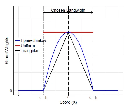
The observations near the cutoff can be seen as a neighborhood, defined as $c-h$ and $c+h$, where $h>0$ is called bandwidth. The observations that are closer to the cutoff receive more weight than those further away, which is achieved by a weighting scheme . These weights are obtained with a kernel function $K(.)$.

There are five steps in the local polynomial estimation:

Select a polynomial order $p$ and a kernel function $K(.)$
Select a bandwidth $h$
For observations above the cutoff, fit a weighted least squares regression, where the estimated intercept from the regression, $\hat{\mu_{+}}$, is an estimate of the point $ \hat{\mu_{+}} = \mathbb{E}[Y_{i}(1)|X_{i} = c] $
For observations below the cutoff, fit a weighted least squares regression, where the estimated intercept from the regression, $\hat{\mu_{-}}$, is an estimate of the point $ \hat{\mu_{-}} = \mathbb{E}[Y_{i}(0)|X_{i} = c] $
Calculate the point estimate $\tau_{SRD} = \hat{\mu_{+}}-\hat{\mu_{-}}$

Therefore, we need to choose the kernel function $K(.)$, the order of the polynomial $p$ and the bandwidth $h$.

Choice of Kernel function

The kernel function assigns positive weights to each observation based on the distance between the score of the observation and the cutoff. There are three types of kernel functions:

The triangular kernel function - it is usually the recommended choice and is defined as $K(u) = (1-|u|)\mathbb{1}(|u| <= 1)$. $\mathbb{1}(.)$ is the indicator function and assigns 0 to all observations with score outside the interval $[c-h, c+h]$ and positive weights to the observations inside this interval. The weight takes the maximum value at $X_{i}=c$ and declines linearly as the score gets farther from the cutoff.
The uniform kernel function - it is a more simple function defined as $K(u) = \mathbb{1}(|u| <= 1)$, which gives the weight 0 to observations with score outside $[c-h, c+h]$ and equal weight to observations inside the interval.
The Epanechnikov kernel function - is defined as $K(u) = (1-u^2)\mathbb{1}(|u| <= 1)$, which gives a quadratic decaying weight to observations inside $[c-h, c+h]$ and 0 to the scores outside this interval.

Types of Kernel Weights

Choice of polynomial order

For a set bandwidth increasing the polynomial order improves the accuracy of the approximation and increases the variability of the treatment effect. Higher-order polynomials tend to produce overfitting of the data and can lead to unreliable results.

Choice of bandwidth and implementation

The bandwidth $h$ defines the width of the interval around the cutoff that is used to fit the local polynomial, therefore $h$ directly affects the estimation and empirical findings. As a general rule, reducing the bandwidth can always improve the accuracy of the approximation. A smaller $h$ reduces the smoothing bias (misspecification error), but also increases the variance of the estimated coefficients, as fewer observations would be available for estimation. Opposingly, a higher bandwidth results in higher smoothing bias and reduces the variance.

In general, there is a trade-off to be made between the bias and the variance. The goal is to minimize the MSE of the local polynomial point estimator, given a choice of $p$ and $K(.)$. The MSE of an estimator is the sum of its squared bias and variance, thus the bias-variance trade-off.

Local polynomial inference

To implement the theory in practice, we can implement a local RD point estimator using the function rdrobust. Besides giving it the data, the function takes three parameters: kernel for specifying the Kernel function, p for specifying the polynomial order and h for setting the bandwidth.

		
#point estimation with triangular kernel, first order polynomial and bandwidth of 20
rdrobust(Y, X, kernel = 'triangular', p = 1, h = 20)

Alternatively, for automatically selecting the bandwidth we can use the function rdbwselect, part of the rdrobust package. It has almost the same parameters as the previous function, except that instead of h it takes the parameter bwselect for setting the bandwidth selection method. It can select an MSE-optimal bandwidth (bwselect = "mserd"), which can either impose the same bandwidth on each side of the cutoff, or set different bandwidths on each side (bwselect = "mstwo").

Apart from an MSE-optimal bandwidth, we can also choose to implement a CER-optimal bandwidth (bwselect = "cerrd"), which minimizes the approximation to the coverage error of the confidence interval of the treatment effect $\tau_{SRD}$.

		
#point estimation with triangular kernel, first order polynomial and CER-optimal bandwidth 
rdbwselect(Y, X, kernel = 'triangular', p = 1, bwselect = "cerrd")

Additionally, we can opt to report all the bandwidth choices. To do this, we replace the bwselect argument with all = TRUE. All the possible bandwidth choices are listed and explained below:

mserd: Bandwidth that minimizes the MSE of the point estimator, where the bandwidth is the same on both sides of the cutoff
msetwo: Bandwidth that minimizes the MSE of the point estimator, where the bandwidths are different on each side of the cutoff
msesum: Bandwidth that minimizes the MSE of the sum of the regression coefficients
msecomb1: Minimum between mserd and msesum
msecomb2: Median of mserd, msetwo and msesum

CER - all are analogous to the previous, but the bandwidths are optimal with respect to the CER of the confidence interval for $\tau_{SRD}$

cerrd
certwo
cersum
cercomb1
cercomb2

Summary

The local polynomial approach in sharp regression discontinuity design (SRD) offers a robust estimation method by focusing on observations around the cutoff, minimizing overfitting issues. The careful selection of the kernel function, polynomial order, and bandwidth is crucial for accurate estimation and reliable results.

The local randomization approach can be seen as an extension of this contuinity-based approach and is discussed in this building block.

Continuity-Based Approach

Introduction