


Introduction
In the last topic, we provided an introduction to the Regression Discontuinity Design and specifically the sharp RDD. Now, we will focus on RDD plots. We can visualize a graphical representation of a RDD by illustrating the relationship between the outcome and the running variable.
Plotting RD Designs can be done with a scatter plot of the observed outcome against the score, where each point would represent one observation. However, simply plotting the raw data makes it hard to see discontinuities in the relationship between score and outcome. To illustrate this, we use the example described in Sharp RD Designs of the Meyersson application. The data is available here: data-link.
A plot with raw data
First we need to open the dataset, rename the columns for better readability and filter the NA values. We do as follows:

#load libraries
library(haven)
library(dplyr)
library(rddensity)
library(rdrobust)
library(ggplot2)

#read data
df <- read_stata("regdata0.dta")

#rename columns
df <- df %>%
  select(vote_share_islam_1994 = vshr_islam1994,
         islamic_mayor_1994 = i94,
         log_pop_1994 = lpop1994,
         no_of_parties_1994 = partycount,
         share_women_hs_1520 = hischshr1520f,
         share_men_hs_1520 = hischshr1520m,
         pop_share_under_19 = ageshr19,
         pop_share_over_60 = ageshr60,
         sex_ratio_2000 = sexr,
         win_margin_islam_1994 = iwm94,
         household_size_2000 = shhs,
         district_center = merkezi,
         province_center = merkezp,
         metro_center = buyuk,
         sub_metro_center = subbuyuk,
         pd_1:pd_67,
         pcode = pcode)

#filter NA
df <- df %>%
  filter(!is.na(share_women_hs_1520),
         !is.na(vote_share_islam_1994),
         !is.na(no_of_parties_1994),
         !is.na(win_margin_islam_1994),
         !is.na(islamic_mayor_1994),
         !is.na(share_men_hs_1520),
         !is.na(household_size_2000),
         !is.na(log_pop_1994),
         !is.na(pop_share_under_19),
         !is.na(pop_share_over_60),
         !is.na(sex_ratio_2000),
         !is.na(district_center),
         !is.na(province_center),
         !is.na(metro_center),
         !is.na(sub_metro_center))
Now let's create a scatter plot of the educational attainment of women against the Islamic vote margin.
plot(df$win_margin_islam_1994,
     df$share_women_hs_1520,
     xlab = "Score",
     ylab = "Outcome",
     col = 1,
     pch = 20,
     cex.axis = 1.5,
     cex.lab = 1.5)
abline(v = 0)
Output:
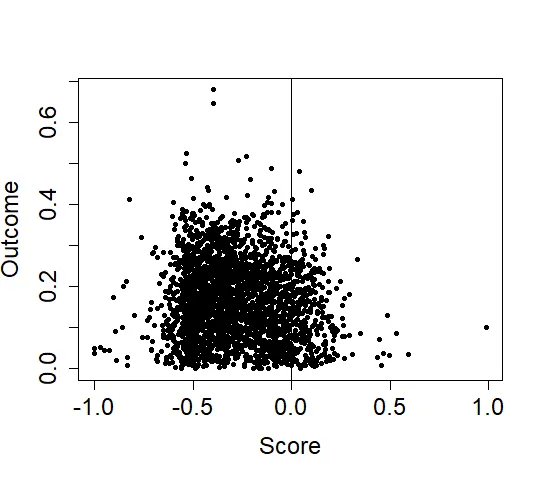
The resulting plot can help to detect outliers and visualize the raw observations, but it makes it hard to effectively visualize the RD design. For instance, we can't see a jump in the values of the outcome by just looking at the raw data.
A typical RD plot
To solve this, we should aggregate the data before plotting. A typical RD plot has two features: - A global polynomial fit, represented by a solid line: a smooth approximation to the unknown regression functions, based on a polynomial fit of the outcome on the score - Local sample means, represented by dots: a non-smooth approximation to the unknown regression functions; they are created by choosing disjoint bins (intervals) of the score followed by a calculation of the mean outcome for observations within each bin and then plotting this average outcome for each bin
Binning the data can reveal patterns that can't be seen when plotting the raw data in a simple scatter plot. There are two important aspects for choosing the bins: location and number.
Location of bins
We can create two different types of bins: - Evenly-spaced (ES): bins that have equal length; however, if observations are not uniformly distributed, each bin might have a different number of observations. - Quantile-spaced (QS): bins that contain roughly the same number of observations but the length may differ; the bins are larger in regions where there are fewer observations.
We create two graphs using 20 evenly-spaced and quantile-spaced bins. To do this we use the rdplot command:
#evenly spaced bins
out <- rdplot(df$share_women_hs_1520,
              df$win_margin_islam_1994,
              nbins = c(20, 20),
              binselect = "es",
              y.lim = c(0,.25),
              title = "Evenly-spaced bins",
              x.label = "Win margin",
              y.label = "Educational attainment")
summary(out)

#quantile spaced bins
out2 <- rdplot(df$share_women_hs_1520,
               df$win_margin_islam_1994,
               nbins = c(20, 20),
               binselect = "qs",
               y.lim = c(0,.25),
               title = "Quantile-spaced bins",
               x.label = "Win margin",
               y.label = "Educational attainment")
summary(out2)
Output:
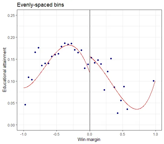
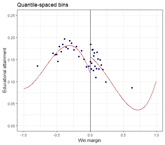
In the evenly-spaced plot there are 3 bins in the interval [0.5, 1], whereas in the quantile-spaced plot the interval is entirely contained by one bin.
Number of bins
There are two methods for choosing the number of bins on both sides of the cutoff, which are noted with $J_{-}$ and $J_{+}$.
Integrated Mean Squared Error (IMSE)
The IMSE method selects the $J_{-}$ and $J_{+}$ values such that it minimizes an asymptotic approximation to the integrated mean-squared error of the local means estimator. The local means estimator is the sum of the expansions of the variance and squared bias. A large number of bins leads to small bias, because the bins are smaller and the local constant fit is better. However, the small bias leads to more variability within the bin, as an increased number of bins would have fewer observations per bin.
We can use the IMSE method with either evenly-spaced or quantile-spaced bins. We use the same rdplot command, but this time there's no need to specify the number of bins with nbins = c(20, 20) option. As long as we set the binselect argument to either es for evenly-spaced or qs for quantile-spaced, rdplot automatically chooses the number of bins according to it.
We first create a plot with evenly-spaced bins and a number of bins that follows the IMSE method.
out3 <- rdplot(df$share_women_hs_1520,
               df$win_margin_islam_1994,
               binselect = "es",
               x.lim = c(-1, 1),
               y.lim = c(0,.25),
               title = "IMSE ES",
               x.label = "Win margin",
               y.label = "Educational attainment")
summary(out3)
Output:
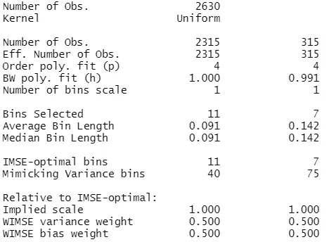
The above output shows the additional descriptive statistics additional to the plot. We notice that there are 2,630 observations in total, with 2,315 to the left of the cutoff and 315 to the right. Because the ES method results in equal length of the bins, each bin has a length equal to the average and the median length for each side: 0.091 for the left side and 0.142 for the right side. The IMSE method gives an optimal number of bins of 11 below the cutoff and of 7 above it.
We now create a plot with quantile-spaced bins.
out4 <- rdplot(df$share_women_hs_1520,
              df$win_margin_islam_1994,
              binselect = "qs",
              x.lim = c(-1, 1),
              y.lim = c(0,.25),
              title = "IMSE QS",
              x.label = "Win margin",
              y.label = "Educational attainment")
summary(out4)
Output:
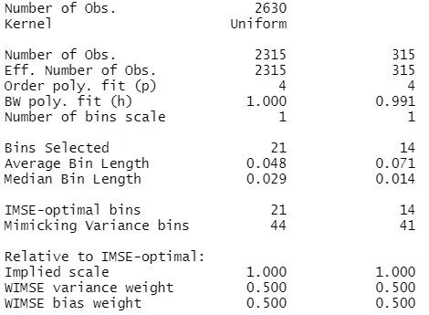
With the quantile-spaced method the resulting number of bins is larger: 21 bins below the cutoff and 14 bins above the cutoff.
Mimicking Variance Method (MV)
The second method chooses the $J_{-}$ and $J_{+}$ values such that the binned means have an asymptotic variability that is approximately equal to the variability of the raw data. This means that the number of bins is chosen in a way that the overall variability of the binned means "mimics" the overall variability in the raw scatter plot.
Again, this method can be used with either method for choosing the bins location. The mimicking variance method results in a larger number of bins than the IMSE method, meaning that we will have a plot with more dots that represent the local means and gives a better sense of the variability in the data.
To create a plot using the MV method with ES bins we use binselect = esmv.
out5 <- rdplot(df$share_women_hs_1520,
              df$win_margin_islam_1994,
              binselect = "esmv",
              title = "MV ES",
              x.label = "Win margin",
              y.label = "Educational attainment")
summary(out5)
Output:
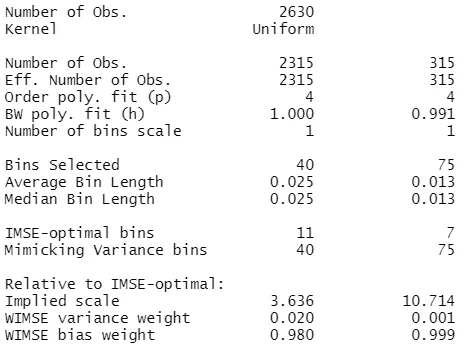
The output shows us that the resulting number of bins is higher that with the IMSE method. Here we have 40 bins below the cutoff with a length of 0.025 and 75 bins above the cutoff with a length of 0.013.
For a plot with QS bins and MV method we use binselect = qsmv.
out6 <- rdplot(df$share_women_hs_1520,
               df$win_margin_islam_1994,
               binselect = "qsmv",
               title = "MV QS",
               x.label = "Win margin",
               y.label = "Educational attainment")
summary(out6)
Output:
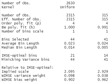
The resulting number of bins below the cutoff is similar to the MV method with ES bins above, but above the cutoff the number of bins in this case is much lower than for ES bins (41 and 75). This happens because the QS bins can be short around the cutoff and long far from the cutoff, which means they can adapt their length to the density of the data. On the other hand, ES bins imposes the same length of the bins, such that the number of bins has to be large to produce small enough bins to mimic the variability of the scatter plot for areas with few observations.
 Summary
There are more methods for choosing the bins for plotting RD designs, depending on the goal. If the goal is to illustrate the variability of the outcome it is better to use MV bins, but if the goal is to test the global features of the regression function, then IMSE method is better. Regardless of the method for number of bins, it is advised to compare both ES and QS bins to highlight the distributional features of the score.
The next topic in this series about Regression Discontuinity describes the local polynomial approach in the context of the Sharp RD Design for estimating the parameter of interest.