Introduction

The purpose of regression analysis is to study the causal effect of a so- called treatment on a variable of interest, for instance the effect of minimum wage increase on unemployment. When the units are assigned randomly to treatment and control groups, the analysis is straightforward. However, if the treatment assignment is not random, then there is need for non-experimental interventions. Regression Discontinuity is a non-experimental research design for analyzing causal effects. The most important feature of this design is that the probability of receiving a treatment changes drastically at a known threshold.

Elements of RD design

The three elements of RD designs (RDD) are:

• Score: each units have a score (also called the running variable)
• Cutoff
• Treatment: a treatment is only assigned to units that have a score above the cutoff (dependent on the specific case, the treatment can be assigned to units below the cutoff)

There are two types of RD designs, sharp and fuzzy RDD. In this building block we cover the sharp design. We start by discussing the setup of a Sharp RDD, followed by a practical example. The fuzzy RDD is covered in this buiding block of the series about RDD.

Sharp RDD setup

The sharp RDD is defined by these features:

• The score is continuously distributed and only has one dimension.
• There is a unique cutoff.
• There is perfect compliance with the treatment assignment: all units with score below the cutoff receive the control condition, all units with score equal or greater than the cutoff receive the treatment.

Suppose we have $n$ units, indexed i = 1, 2, …, n, and each unit has a score $X_{i}$ and $c$ is the known cutoff.

• All units with $X_{i} >= c$ are assigned to the treatment condition
• All units with $X_{i} < c$ are assigned to the control condition.

The treatment assignment is denoted with $T_{i}$ and is defined as $T_{i} = \mathbb{1}(X_{i} >= c)$, where $\mathbb{1}(.)$ is the indicator function which is equal to 1 if the condition in the brackets is satisfied, and equal to 0 otherwise.

We need to make a distinction between being assigned to the treatment and receiving or complying with the treatment. In the sharp RD design, the treatment condition assigned is the same with the treatment actually received by the units.

Treatment probability

We go back to the defining feature of any RDD: the conditional probability of actually receiving treatment changes discontinuously at the cutoff. For the sharp design, the probability changes from 0 to 1 at the cutoff, as we can see in the graph below.

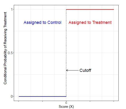
The probability of receiving treatment given a score is denoted with $P(T_{i} = 1|X_{i} = x)$.

Potential outcomes

Every unit is assumed to have two potential outcomes, one for treatment $Y_{i}(1)$ and one for control $Y_{i}(0)$. However, only one of them can be observed, so if unit $i$ receives treatment we observe $Y_{i}(1)$, while if unit $i$ receives the control condition we only observe $Y_{i}(0)$. This leads to the **fundamental problem of causal inference**: the treatment effect at the individual level is fundamentally not knowable.

The observed outcome is defined as follows $Y_{i} = (1-T_{i})*Y_{i}(0) + T_{i}*Y_{i}(1)$ and can take two values:

• $Y_{i}(0)$, if $X_{i} < c$, because $T_{i} = 0$
• $Y_{i}(1)$, if $X_{i} >= c$, because $T_{i} = 1$

Additionally, the average potential outcomes given the score are given by the conditional expectation function, also called regression function, denoted by $\mathbb{E}[Y_{i}|X_{i}]$ and can take two values:

• $\mathbb{E}[Y_{i}(0)|X_{i}]$, if $X_{i} < c$
• $\mathbb{E}[Y_{i}(1)|X_{i}]$, if $X_{i} >= c$

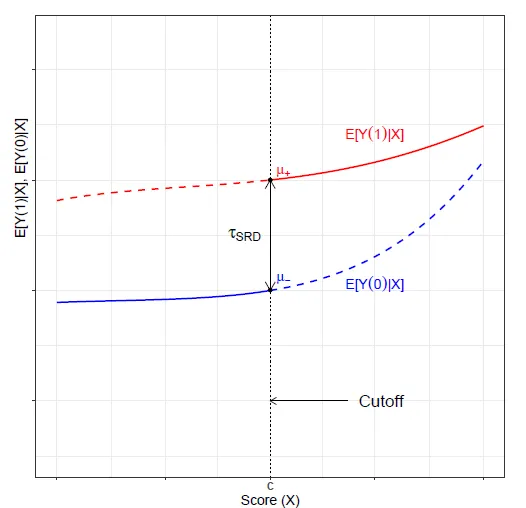
The plot below shows us that the function $\mathbb{E}[Y_{i}(0)|X_{i}]$ is observed for units with score lower than the cutoff (blue line), whereas the function $\mathbb{E}[Y_{i}(1)|X_{i}]$ is observed for units with score higher than the cutoff (red line).

Treatment effect

Remember that sharp RDD implies that units from treatment and control groups can’t have the same score $X_{i}$. The graph above shows that we can’t observe both red and blue lines for the same value of the score, except for the cutoff, where we almost see both curves.

Suppose we have a unit with the score equal to $c$ and one unit with a score just below $c$. Even if the the units would be very similar, the difference is given by their treatment condition and we could calculate the vertical distance at $c$. As shown in the above graph, the vertical distance between the two points is the sharp RD treatment effect, which is defined as: \(\tau_{SRD} = \mathbb{E}[Y_{i}(1) - Y_{i}(0)|X_{i} = c]\)

This parameter can be interpreted as the average treatment effect on the treated and can answer the question: what would be the average outcome change for units with a score level $X_{i}=c$ if we switched their status from control to treated?

Practical example

To illustrate the theory with a practical example, we use the example given by Cattaneo, Idrobo & Titiunik (2020) in their paper on regression discontinuity. Meyersson (2014) studied the effect of Islamic parties' control of local governments on the educational attainment of young women. There are two possibilities: municipalities in which the support for Islamic parties is high and results in the election of an Islamic mayor, and municipalities in which the support for Islamic parties is weaker and it results in the election of a non-Islamic mayor (also called secular).

Sharp RDD can be configured as follows:

• The unit of analysis is the municipality
• The **score $X_{i}$** is the Islamic margin of victory - the difference between the vote percentage of the largest Islamic party and the vote percentage of the largest non-Islamic opponent
• The **treatment group $T_{i} = 1$** consists of the municipalities that elected an Islamic party mayor
• The **control group $T_{i} = 0$** consists of municipalities that elected a non-Islamic party mayor
• The **outcome $Y_{i}$** is the educational attainment of women, measured as the percentage of women (aged 15 to 20) who had completed high school by 2000

Local nature of RD effects

The $\tau_{SRD}$ parameter is causal, because it captures the average difference in potential outcomes between treatment and control. This causal effect is local in nature because the difference is calculated at a single point of a continuous random variable $X_{i}$. However, this treatment effect has limited external validity, meaning that the effect is not representative of treatment effects that occur for scores away from the cutoff. Thus, it may not be informative for values of $X_{i}$ different from $c$, and it is only the average effect of the treatment for units **local to the cutoff**.

To extrapolate the RD treatment effect, certain assumptions should be imposed about:

• the regression functions near the cutoff
• local independence assumptions
• exploiting specific features of the design, like imperfect compliance
• the presence of multiple cutoffs

Summary

RDD is a non-experimental research design used to analyze causal effects. In this first building block of a series on Regression Discontuinity Design, we discussed the sharp RDD. The sharp RD relies on a few important features, like a continuous distribution of the score that has only one dimension, existence of a unique cutoff and perfect compliance with treatment assignment. The sharp RD treatment effect is the average difference in potential outcomes between treatment and control at the cutoff.

In the next building block, we will dive deeper into the RDD subject by discussing Regression Discontuinity plots.

See also

A Practical Introduction to Regression Discontinuity Designs: Foundations - Cattaneo, Idrobo & Titiunik (2020)