


Overview
The main purpose of the kableExtra package is to simplify the process of creating tables with custom styles and formatting in R. In this building block, we will provide an example using some useful functions of kableExtra to improve the output of the modelsummary package and create a table in LaTeX format suitable for a publishable paper.
The starting point is the final output of our modelsummary building block, which is a replication of Table 1 of Eiccholtz et al. (2010). This table presents the results of a model investigating how green building certification impacts rental prices of commercial office buildings.
The following kableExtra functions will be covered to get to a formatted table that can be inserted into a research paper or slide deck that is built using LaTeX:
- Output in LaTex format
- Exporting the table to a file
- Specifying the column alignment within the table
- Add rows to the table to designate which fixed effects are included in each regression specification
- Add a row that specifies the dependent variable in the regression
- Formatting and grouping rows of regression coefficients
Load packages and data
To begin, let's load the necessary packages and data:

# Load packages
library(modelsummary)
library(dplyr)
library(fixest)
library(stringr)
library(knitr)
library(kableExtra)

# Load data
data_url <- "https://github.com/tilburgsciencehub/website/blob/master/content/topics/Visualization/Reporting_tables/ReportingTables/data_rent.Rda?raw=true"
load(url(data_url)) #data_rent is loaded now
The modelsummary table
- 'models' is a list which consists of five regression models (regression 1 to 5). For a detailed overview and understanding of these regressions, please refer to the
modelsummarybuilding block. cm2andgm2represent the variable names and statistics included in the regression table, respectively.
cm2 = c('green_rating'    = 'Green rating (1 $=$ yes)',
        'energystar'    = 'Energystar (1 $=$ yes)',
        'leed'    = 'LEED (1 $=$ yes)',
        'size_new'    = 'Building size (millions of sq.ft)',
        'oocc_new' = 'Fraction occupied',
        'class_a' = 'A (1 $=$ yes)',
        'class_b' = 'B (1 $=$ yes)',
        'net' = 'Net contract (1 $=$ yes)',
        'age_0_10' = '<10 years',
        'age_10_20' = '10-20 years',
        'age_20_30' = '20-30 years',
        'age_30_40' = '30-40 years',
        'renovated' = 'Renovated (1 $=$ yes)',
        'story_medium' = 'Intermediate (1 $=$ yes)',
        'story_high' = 'High (1 $=$ yes)',
        'amenities' = 'Amenities (1 $=$ yes)')

gm2 <- list(
    list("raw" = "nobs", "clean" = "Sample size", "fmt" = 0),
    list("raw" = "r.squared", "clean" = "$R^2$", "fmt" = 2),
    list("raw" = "adj.r.squared", "clean" = "Adjusted $R^2$", "fmt" = 2))

msummary(models,
         vcov = "HC1",
         fmt = fmt_statistic(estimate = 3, std.error = 3),
         #stars  = c('*' = .1, '**' = 0.05, '***' = .01),
         estimate = "{estimate}",
         statistic = "[{std.error}]{stars}",
         coef_map = cm2,
         gof_omit = 'AIC|BIC|RMSE|Within|FE',
         gof_map = gm2)
| (1) | (2) | (3) | (4) | (5) | |
|---|---|---|---|---|---|
| Green rating (1 = yes) | 0.035 | 0.033 | 0.028 | ||
| [0.009] | [0.009] | [0.009] | |||
| Energystar (1 = yes) | 0.033 | ||||
| [0.009] | |||||
| LEED (1 = yes) | 0.052 | ||||
| [0.036] | |||||
| Building size (millions of sq.ft) | 0.113 | 0.113 | 0.102 | 0.110 | 0.110 |
| [0.019] | [0.019] | [0.019] | [0.021] | [0.021] | |
| Fraction occupied | 0.020 | 0.020 | 0.020 | 0.011 | 0.011 |
| [0.016] | [0.016] | [0.016] | [0.016] | [0.016] | |
| A (1 = yes) | 0.231 | 0.231 | 0.192 | 0.173 | 0.173 |
| [0.012] | [0.012] | [0.014] | [0.015] | [0.015] | |
| B (1 = yes) | 0.101 | 0.101 | 0.092 | 0.083 | 0.083 |
| [0.011] | [0.011] | [0.011] | [0.011] | [0.011] | |
| Net contract (1 = yes) | -0.047 | -0.047 | -0.050 | -0.051 | -0.051 |
| [0.013] | [0.013] | [0.013] | [0.013] | [0.013] | |
| <10 years | 0.118 | 0.131 | 0.131 | ||
| [0.016] | [0.017] | [0.017] | |||
| 10-20 years | 0.079 | 0.084 | 0.084 | ||
| [0.014] | [0.014] | [0.014] | |||
| 20-30 years | 0.047 | 0.048 | 0.048 | ||
| [0.013] | [0.013] | [0.013] | |||
| 30-40 years | 0.043 | 0.044 | 0.044 | ||
| [0.011] | [0.011] | [0.011] | |||
| Renovated (1 = yes) | -0.008 | -0.008 | -0.008 | ||
| [0.009] | [0.009] | [0.009] | |||
| Intermediate (1 = yes) | 0.010 | 0.010 | |||
| [0.009] | [0.009] | ||||
| High (1 = yes) | -0.027 | -0.027 | |||
| [0.015] | [0.015] | ||||
| Amenities (1 = yes) | 0.047 | 0.047 | |||
| [0.007] | [0.007] | ||||
| Sample size | 8105 | 8105 | 8105 | 8105 | 8105 |
| R2 | 0.71 | 0.71 | 0.72 | 0.72 | 0.72 |
| Adjusted R2 | 0.69 | 0.69 | 0.69 | 0.69 | 0.69 |
Output in LaTex format
We want the table to be outputted in LaTeX format now. We set the output argument to latex in the msummary() function. This generates LaTeX code that can be directly copied and pasted into a LaTeX document.
msummary(models,
         vcov = "HC1",
         fmt = 3,
         estimate = "{estimate}",
         statistic = "[{std.error}]",
         coef_map = cm2,
         gof_omit = 'AIC|BIC|RMSE|Within|FE',
         gof_map = gm2,
         output = "latex",
         escape = FALSE
         )
 Tip
TipWhen escape = FALSE, any special characters that are present in the output of msummary() will not be modified or escaped. This means that they will be printed exactly as they appear in the output, without any changes or substitutions. On the other hand, if escape = TRUE, then any special characters that are present in the output will be replaced with the appropriate LaTeX commands to render them correctly in the final document.
Export the table to a file
To save this LaTex code to a .tex file, we can use the cat() function. The file argument specifies the name of the file we want the output to be printed to: my_table.tex. Not including any file argument will print the output to the console.
msummary(models,
         vcov = "HC1",
         fmt = 3,
         stars  = c('*' = .1, '**' = 0.05, '***' = .01),
         estimate = "{estimate}",
         statistic = "[{std.error}]",
         coef_map = cm2,
         gof_omit = 'AIC|BIC|RMSE|Within|FE',
         gof_map = gm2,
         output = "latex",
         escape = FALSE
         ) %>%
  cat(.,file="my_table.tex")
The %>% operator is being used to pipe the output of msummary() into the cat() function. Specifically, the dot (.) is a placeholder for the output of the previous function in the pipeline, which in this case is msummary().
TipThe LaTex file requires the following packages loaded in the header:
LaTex
\usepackage{booktabs}
\usepackage{siunitx}
\usepackage{bbding}
Specify the column alignment
You can customize the horizontal alignment of the table columns by including the align argument within the msummary() function. By setting align = "lcccc", you can specify the alignment for each column as follows:
- The first column, containing the variable names, will be left-aligned (l).
- The second to fifth columns, displaying the coefficients, will be centered (c).
msummary(models,
          vcov = "HC1",
          fmt = 3,
          estimate = "{estimate}",
          statistic = "[{std.error}]",
          coef_map = cm2,
          gof_omit = 'AIC|BIC|RMSE|Within|FE',
          gof_map = gm2,
          align="lccccc",
          output = "latex",
          escape = FALSE
          )
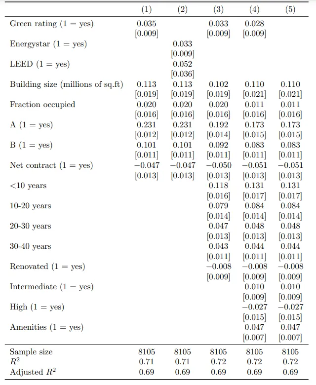
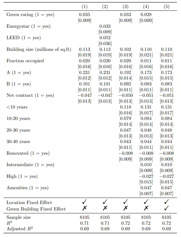
Add rows designating fixed-effects specification
In this step, we will integrate additional rows in the regression table to indicate the inclusion of fixed effects in each model.
Creating a tibble
First, the additional rows are specified in a tibble. Within the tibble:
- There are two columns: term and "(1)", "(2)", "(3)", "(4)", "(5)".
- The two rows specify the two kind of Fixed Effects: Location Fixed Effect & Green Building Fixed Effect. In these rows, it is specified for each regression model whether these fixed effects are included: "Checkmark" indicates they are included, and "XSolidBrush" indicates they are not included.
library(tibble)

rows <- tribble(~term,          ~"(1)", ~"(2)", ~"(3)",~"(4)", ~"(5)",
                'Location Fixed Effect', '\\Checkmark',   '\\Checkmark', '\\Checkmark', '\\Checkmark', '\\Checkmark',
                'Green Building Fixed Effect', '\\XSolidBrush',   '\\XSolidBrush', '\\XSolidBrush', '\\XSolidBrush', '\\Checkmark'
)
Position of Fixed Effect rows in table
To insert the fixed effect rows at the appropriate location in the table (between the estimates and statistics), we use the attr() function. These rows should be placed at row 33 and 34.
R
attr(rows, 'position') <- c(33, 34)
add_rows
To include the tibble with the fixed effect rows in the final table, we use the add_rows = rows argument within the msummary() function. Note that rows refers to the name of our tibble.
row_spec
To distinguish the fixed effect rows from the summary statistics, we can add a horizontal line below the fixed effect rows using the row_spec() function after modelsummary(), using the pipe operator.
Here is the msummary() function incorporating the mentioned arguments to generate the regression table with fixed effect rows:
msummary(models,
         vcov = "HC1",
         fmt = 3,
         estimate = "{estimate}",
         statistic = "[{std.error}]",
         coef_map = cm2,
         gof_omit = 'AIC|BIC|RMSE|Within|FE',
         gof_map = gm2,
         add_rows = rows,
         align="lccccc",
         output = "latex",
         escape = FALSE
         ) %>%
    row_spec(34, extra_latex_after = "\\midrule") %>%
    cat(., file = "my_table.tex")
The table generated using the previous code is displayed below. As you can see, fixed effect rows are added now!
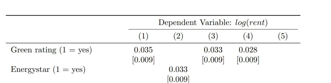
Add header
To include a header above the existing column headers of the regression table, we can use the add_header_above() function.
- The name of the header should be provided as a character string.
- To span the header across columns 2 to 6 while excluding the first column, we can set the header value to 5.
msummary(models,
         vcov = "HC1",
         fmt = 3,
         estimate = "{estimate}",
         statistic = "[{std.error}]",
         coef_map = cm2,
         gof_omit = 'AIC|BIC|RMSE|Within|FE',
         gof_map = gm2,
         add_rows = rows,
         align="lccccc",
         output = "latex",
         escape = FALSE
         ) %>%
    add_header_above(c(" " = 1,
                       "Dependent Variable: $log(rent)$" = 5),
                     escape = FALSE
    )
    cat(., file = "my_table.tex")
The LaTeX output displays the header as follows:
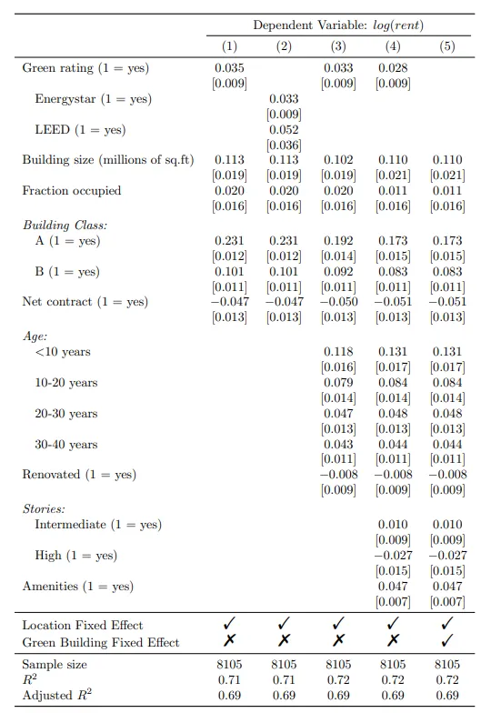
Group rows
Add a labeling row
We can use the pack_rows() function to insert labeling rows and group variables into categories. In our case, we have three categories: Building Class, Age and Stories.
Within pack_rows(), we provide the category name along with the first and last row numbers for the variables that belong to that category. Additionally, we can specify the formatting for the category name, such as printing it in italic text instead of bold.
Indent subgroups
To indicate that Energystar and LEED are subgroups of the variable Green rating (row 1), we can use the add_intent() function. This function allows us to indent specific rows.
msummary(models,
         vcov = "HC1",
         fmt = 3,
         estimate = "{estimate}",
         statistic = "[{std.error}]",
         coef_map = cm2,
         gof_omit = 'AIC|BIC|RMSE|Within|FE',
         gof_map = gm2,
         add_rows = rows,
         align="lccccc",
         output = "latex",
         escape = FALSE
         ) %>%
    pack_rows("Building Class:", 11, 13, italic = TRUE, bold = FALSE) %>%
    pack_rows("Age:", 17, 24, italic = TRUE, bold = FALSE) %>%
    pack_rows("Stories:", 27, 30, italic = TRUE, bold = FALSE) %>%
    add_indent(3) %>%
    add_indent(5) %>%
    row_spec(34, extra_latex_after = "\\midrule") %>%
    cat(., file = "my_table.tex")
 Summary
The kableExtra package provides powerful tools for creating attractive and publication-ready tables in R. By combining it with the modelsummary package, we can generate informative and visually appealing regression tables for our research papers or reports.
This example shows how to use some kableExtra functions to improve a standard modelsummary table and have it outputted in LaTex format. The functions covered include how export the table in LaTeX format, specify column alignment, add fixed effect rows, add a header, and group rows.