


Overview
In the context of non-feasible randomized controlled experiments, we previously discussed the importance of the difference-in-difference (DiD) approach for causal inference. While calculating treatment effects using the difference-in-means method is a starting point, it lacks sufficient grounds for reliable inference. To obtain more robust results, it is crucial to estimate treatment effects through regression analysis with the appropriate model specification. Regression models allow for controlling confounding variables, accounting for unobserved heterogeneity, and incorporating fixed effects, leading to more accurate and meaningful interpretations of treatment effects. Next, we’ll dig a little deeper into the merits of the regression approach and how to carry out the estimation in R using an illustrative example.
Why Regression Approach?
- Get standard error of the estimate - In order to assess the statistical significance of the effect, it is crucial to obtain the standard error of the estimate. This measure quantifies the variability in the observed treatment effect and provides a range within which the true treatment effect is likely to fall. By calculating the standard error, we can determine whether the observed effect is statistically significant or if it could have occurred by chance alone. This information is essential in drawing reliable conclusions from our analysis. - Additionally, it is important to cluster standard errors when dealing with data that might exhibit clustering or dependence. Clustering occurs when observations within a particular group or cluster are more similar to each other than to observations in other clusters. By clustering standard errors, we appropriately account for this correlation structure, ensuring that our statistical tests and confidence intervals are valid. Failing to cluster standard errors can lead to inaccurate inference and potentially erroneous conclusions.
- Can add extra control variables into the regression - One advantage of the regression approach is the ability to include additional control variables in the analysis. These control variables can serve as "usual" controls, representing factors that may influence the outcome variable but are not the primary focus of the study. By including these controls, we can account for potential confounding variables and improve the accuracy of our estimation of the treatment effect. - Moreover, regression analysis allows for the inclusion of fixed effects. Fixed effects refer to variables that capture individual-specific or group-specific characteristics that are constant over time. By including fixed effects, we can account for unobserved heterogeneity across individuals or groups, thereby controlling for time-invariant factors that might affect the outcome variable. This approach is particularly valuable in natural or quasi-experimental settings where random assignment of treatments may not be feasible.
- Can use log(y) as the dependent variable - When using the regression approach, one option is to use the logarithm of the dependent variable (log(y)) instead of the raw variable. This transformation has several benefits. It can help mitigate issues related to the distributional properties of the outcome variable, such as skewness or heteroscedasticity, which can violate the assumptions of linear regression models. Taking the logarithm can often lead to a more symmetrical and normally distributed dependent variable, improving the validity of the statistical analysis. - Additionally, interpreting the treatment effect in terms of a percentage change becomes possible when using log(y) as the dependent variable. In this case, the estimated treatment effect represents the percentage change in the outcome variable that can be attributed to the treatment. This interpretation is particularly useful in situations where the relative impact of the treatment is of interest, as it provides a meaningful measure of the treatment's effectiveness.
By considering the context and benefits outlined above, the regression approach proves to be advantageous for assessing causal relationships. It enables us to obtain standard errors, account for additional control variables, and interpret treatment effects in a meaningful way, contributing to a more comprehensive and robust analysis of the treatment's impact.
An illustrative example (Continued)
In the previous topic, we introduced an example to illustrate how to obtain the difference-in-means table for a 2 x 2 DiD design. This example looks into the effect of the Q&A on subsequent ratings using a cross-platform identification strategy with Goodreads as the treatment and Amazon as the control group. We have 2 groups (Amazon vs Goodreads) and 2 time periods (pre Q&A and post Q&A).
The effect can be estimated with the following regression equation. You can find all the analysis code in this Gist.
$$ rating_{ijt} = \alpha+ \lambda POST_{ijt}+\gamma Goodreads+\delta (POST_{ijt}* Goodreads_{ij})+\eta_j +\tau_t+\epsilon_{ijt} $$
where, - $POST$ is a dummy equal to 1 if the observation is after Q&A launch - $Goodreads$ is a dummy equal to 1 if the observation is from the Goodreads platform and 0 if from Amazon - $\eta$: Book fixed effects - $\tau$: Time fixed effects
Before estimating the regression, it is crucial to check whether the parallel trends assumption holds which suggests that, in the absence of the treatment, both the treatment and control groups would have experienced the same outcome evolution. We also implicitly assume that the treatment effect is constant between the groups over time. Only then can we interpret the DiD estimator (treatment effect) as unbiased.
To check for parallel trends, we can visualise the average outcome for both groups over time before and after the treatment.
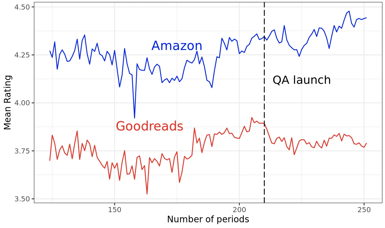
Here we see that both groups follow similar trends prior to the treatment which hints at the plausibility of the parallel trends assumption in this case.
Now let’s estimate a simple regression to obtain the treatment effect.

# Simple linear regression
model_1<- lm(rating ~ goodr*qa, data = GoodAma)
tidy(model_1, conf.int = TRUE)
However, there might be time-varying and group-specific factors that may affect the outcome variable which requires us to estimate a two-way fixed effects (TWFE) regression. Check out this topic to learn more about the TWFE model, and this topic to learn more about the fixest package.
# load packages
library(fixest)
# time fixed effects only model

model_2<- feols(rating ~ goodr*qa
                  |
                  year_month,
                data = GoodAma)

tidy(model_2, conf.int = TRUE)

# both time and book fixed effects model

model_3<- feols(rating ~ goodr*qa
                |
                year_month + asin,
                data = GoodAma)
tidy(model_3, conf.int = TRUE)
Clustered Standard Errors
Clustering standard errors accounts for the potential correlation or dependence within clusters of data, which is commonly encountered in DiD designs. In this example, we might want to cluster standard errors at the book level this way using the cluster argument.
# time and book fixed effects with clustered SE
model_4<- feols(rating ~ goodr*qa
                |
                year_month + asin,
                cluster = c("asin"),
                data = GoodAma)
tidy(model_4, conf.int = TRUE)
Clustering standard errors recognizes that observations within a cluster, such as products or books, may be more similar to each other than to observations in other clusters. This correlation arises due to unobserved factors specific to each cluster that can affect the outcome variable. Failure to account for this correlation by clustering standard errors may result in incorrect standard errors, leading to invalid hypothesis tests and confidence intervals.
Now let’s wrap up this example by comparing all the regression results obtained so far.
| (1) | (2) | (3) | (4) | |
|---|---|---|---|---|
| Treated (1 = Goodreads) | -0.465 | -0.452 | -0.372 | -0.372 |
| [0.003]*** | [0.008]*** | [0.011]*** | [0.047]*** | |
| After (1 = post QA) | 0.106 | 0.021 | 0.029 | 0.029 |
| [0.002]*** | [0.004]*** | [0.003]*** | [0.024] | |
| Treatment Effect (treated x after) | -0.095 | -0.107 | -0.152 | -0.152 |
| [0.004]*** | [0.012]*** | [0.009]*** | [0.029]*** | |
| Num.Obs. | 1469344 | 1469344 | 1469344 | 1469344 |
| R2 | 0.045 | 0.048 | 0.135 | 0.135 |
| R2 Adj. | 0.045 | 0.048 | 0.130 | 0.130 |
| FE: year_month | X | X | X | |
| FE: asin | X | X | ||
 Tip
TipUse the modelsummary package to summarise and export the regression results neatly and hassle-free. Check out this topic to help you get started!
In model 4, the estimated treatment effect is substantially larger compared to the previous models, emphasizing the significance of selecting an appropriate model specification. By incorporating fixed effects and clustering standard errors, we effectively control for potential unobserved heterogeneity, ensuring more reliable and valid inference. The inclusion of fixed effects allows us to account for time-invariant factors that may confound the treatment effect, while clustering standard errors addresses the within-cluster dependence commonly encountered in Difference-in-Differences (DiD) designs. This improved model specification enhances the robustness of the estimated treatment effect and strengthens the validity of our conclusions, emphasizing the importance of these methodological considerations in conducting rigorous empirical analyses.
 Summary
- The regression approach in the difference-in-difference (DiD) analysis offers several advantages: obtain standard errors, include control variables and perform log transformation on the dependent variable.
- Time and group fixed effects can be incorporated in the regression analysis to account for time-varying and group-specific factors that may affect the outcome variable. We carry out this two-way fixed effects (TWFE) estimation using the
feols()function from thefixestpackage. - Clustering standard errors is important in DiD designs to address potential correlation or dependence within clusters of data. This can be done using the
clusterargument.
To Know More
- De Chaisemartin, C., & d'Haultfoeuille, X. (2022). Two-way fixed effects and differences-in-differences with heterogeneous treatment effects
- Cunningham, S. (2021). Causal inference: The mixtape. Yale university press.
- Cluster-robust inference: A guide to empirical practice