Overview

The first step before estimating an OLS regression is to validate the model assumptions to ensure the estimates are reliable and the inference drawn is valid.

To illustrate how to check for model assumptions with an example, we use the built-in cars dataset which includes 50 data points of a car’s stop distance at a given speed. Since the dimensions are in miles per hour and foot, we first convert it into kilometer per hour and meter, respectively.

Then, we estimate a linear model and evaluate its properties with autoplot function from the broom package.

Example code

library(ggplot2)
library(ggfortify)
library(broom)
library(dplyr)

data(cars) # import built-in car dataset
cars$speed_kmh <- cars$speed * 1.60934  # convert miles per hour to kilometer per hour
cars$dist_m <- cars$dist * 0.3048  # convert foot to meters

# estimate linear model
mdl_cars <- lm(dist_m ~ speed_kmh, data=cars)

# check linear model assumptions
autoplot(
  mdl_cars,
  which = 1:3,
  nrow = 1,
  ncol = 3
)

Outputs

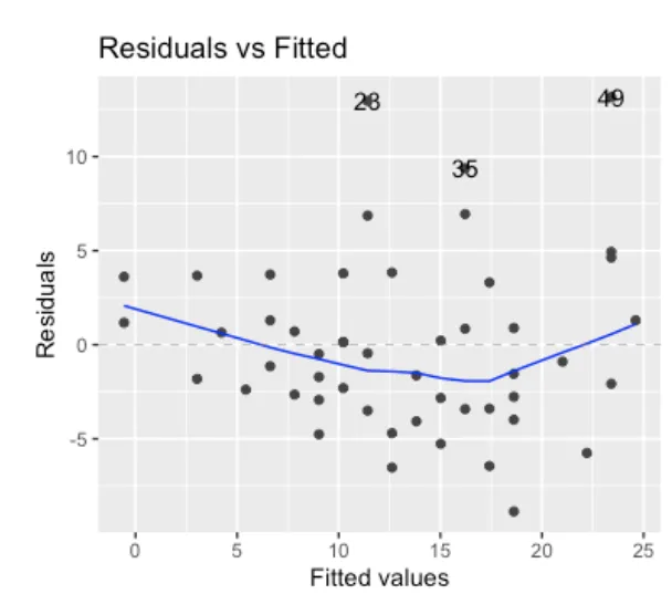
• Residuals vs Fitted: Residuals indicate the difference between the predicted and the actual value. The residuals vs fitted plot shows the residuals and the data points should center around the horizontal axis (i.e., the mean of the residuals is 0). The equally spread residuals around the horizontal line without distinct patterns are a good indication of having the linear relationships. Although the line goes a little downward around the middle, it does not look worrisome at first sight. The linearity assumption seems to hold reasonably well.

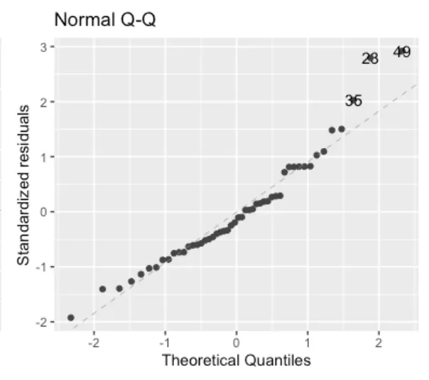
• Normal Q-Q: Another requirement is that the residuals are approximately normally distributed. This means that if you would plot the distribution of all residuals it would look like a bell-shaped distribution (also known as Gaussian distribution). This is the case if the data points in the QQ-Plot are close to the diagonal. Here, we find that record 23, 35, and 49 are somewhat higher than expected (the right tail).

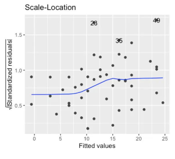
• Scale-Location: Finally, the scale-location plot shows the standardized residuals for all fitted values. The homoskedasticity assumption states that the error term should be the same across all values of the independent variables. Hence, we should check here if there is any pattern that stands out. In our case, this happens to be the case as the blue line stays rather flat. It would, however, be troublesome if the error value increases for higher speed values(i.e. if there is a “fanning out” pattern).