Overview

In the social sciences, regression analysis is a popular tool to estimate relationships between a dependent variable and one or more independent variables. It is a way to find trends in data, quantify the impact of input variables, and make predictions for unseen data.

In this topic, we illustrate how to estimate a model, identify outliers, plot a trend line, and make predictions.

Code

Estimate the Model

Linear regression (lm) is suitable for a response variable that is numeric. For logical values (e.g., did a customer churn: yes/no), you need to estimate a logistic regression model (glm). The code sample below estimates a model, checks the model assumptions, and shows the regression coefficients.

• Model transformations can be incorporated into the formula. For example: formula = log(y) ~ I(x^2).
• The coefficients (coefficients(mdl)), predictions for the original data set (fitted(mdl)), and residuals (residuals(mdl)) can be directly derived from the model object.
• A concrete example of how to evaluate model assumptions (mean of the residuals is 0, residuals are normally distributed, homoscedasticity) can be found in this topic.

library(broom)

# estimate linear regression model
# to estimate a logistic regression model use:
# glm(formula = y ~ x, data = data, family = binomial)
mdl <- lm(formula = y ~ x, data = data)

# check model assumptions
autoplot(
  mdl,
  which = 1:3,
  nrow = 1,
  ncol = 3
)

# show regression coefficients
summary(mdl)

Identify Outliers

Compute the leverage of your data records and influence on mdl to identify potential outliers.

library(dplyr)
leverage_influence <- mdl %>%
    augment() %>%
    select(y, x, leverage = .hat, cooks_dist = .cooksd) %>%
    arrange(desc(cooks_dist)) %>%

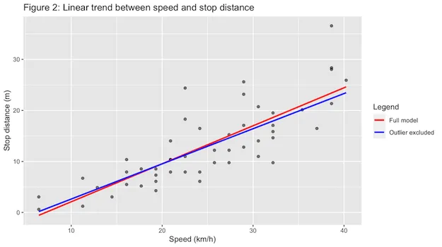
Plot a Trend Line

Plot a scatter plot of two numeric variables and add a linear trend line on top of it.

library(ggplot2)

ggplot(data = data, aes(x, y)) +
geom_points() +
geom_smooth(method = "lm", se = FALSE)

Make Predictions

Given a linear regression model (mdl), make predictions for unseen input data (explanatory_data). Note that for multiple linear regression models, you need to pass an explanatory_data object with multiple columns.

explanatory_data <- c(..., ..., ...)

prediction_data <- explanatory_data %>%
  mutate(
    y = predict(
      mdl,
      explanatory_data,
      type = "response"
    )
  )

# See the result
prediction_data

Export Model Output

You can export your model output using stargazer. This package will create a nicely-formatted regression table for you in a variety of formats. You can learn more about it here.

Convert regression coefficients of mdl_1 and mdl_2 into a HTML file that can be copied into a paper.

library(stargazer)

stargazer(mdl_1, mdl_2,
          title = "Figure 1",
          column.labels = c("Model 1", "Model 2"),
          type="html",
          out="output.html"
          )

Exporting your findings in Stata

Alternatively, you can do your regression analysis on Stata. First, you should clear your working directory. With the command “sysuse auto”, we download an example data file provided by Stata itself.

-Stata-

clear all

* First,let's install the necesary package

ssc install estout, replace

* By typing the command below, you can open an example dataset provided by Stata :

sysuse auto

// Using esttab
eststo clear
* First regression :

eststo: regress price weight mpg

* Second regression

eststo: regress price weight mpg foreign

* Generating a table for the two regression results that we generated :

esttab

eststo clear


// Using outreg2 : Alternatively, you can export your results to an excel, pdf or doc file using outreg2 commandFir


clear all

* First,let's install the necesary package

ssc install outreg2, replace

sysuse auto

* First regression :

regress price weight mpg
outreg2 using RegressionResults.doc, replace ctitle(Model 1)

* Second regression

eststo: regress price weight mpg foreign
outreg2 using RegressionResults.doc, append ctitle(Model 2)

Example

This cars example outlines how to run, evaluate, and export regression model results for the cars dataset. In particular, it analyzes the relationship between a car’s speed and the stop distance.