


Overview
Here we introduced matching where we specifically discussed exact matching, the method in which individuals are paired on one or more identical characteristics.
Now we will continue with approximate matching, where pairs are made on similar but not identical characteristics. It is again a way to adjust for differences when treatment is non-random. Important to mention is that this method is only relevant for selection on observables, which means you should be able to identify the confounders (and have data on them!) that are biasing the effect. We focus on Propensity Score Matching specifically and provide a code example in R.
Curse of dimensionality
Exact matching requires an untreated unit with the precise similar value on each of the observed characteristics to be a good counterfactual for the treated units. The curse of dimensionality means that when there is a large number of variables you are matching treated and untreated units, or when some variables are continuous, there might be no appropriate counterfactual left (that has all the same values on all these covariates). This can be an issue in finite samples, where you have too many covariates to match and not enough data.
Approximate matching offers a solution; it reduces the dimensionality by defining a distance metric on characteristic X and pair units based on this distance rather than the value of X. As the sample gets larger, approximate matching method results will all tend towards exact matching.
Approximate matching methods
 Summary
Common methods of approximate matching include:
-
Nearest-neighbour matching: Pairs each treated unit with the "nearest" untreated unit based on defined characteristics.
-
Kernel matching: Estimates the counterfactual outcome of the treated unit by averaging outcomes of nearby control units.
-
Propensity score matching: Uses the propensity score, representing the probability of treatment assignment given observed covariates.
The guide of Glen Waddel is a good resource that discusses these types in more detail.
As the sample size increases, different matching estimators will yield similar results. However, their performance varies in finite samples. The choice depends on your data. Glen Waddel also gives a broader discussion on this and some points to consider when choosing the method.
Propensity score matching
Propensity score matching addresses the curse of dimensionality by matching on the "propensity score", representing the probability of being assigned to the treatment group, conditional on the particular covariates $X$:
$P(X_{i}) ≡ Pr(D_i = 1 | X_i)$
By controlling for these propensity scores, you compare units that, based solely on their observable characteristics, had similar probabilities of getting the treatment. This mitigates the selection bias; the remaining variation in the outcome variable can then be assigned as being due to the treatment only.
 Tip
TipWhen conditional independence holds true given $X$, it also holds true when conditioned on the propensity score. This famous result by Rosenbaum and Robin (1983) is useful because while $X$ may be high-dimensional, the propensity score is one-dimensional. Consequently, matching on the propensity score increases the likelihood of finding common support between treatment and control groups, facilitating better and closer matches.
Practical example of PSM
Setting
We will use the second example of Imbens (2015) to show matching in practice. Find context on the example in part B section 6.2. The authors examine the effect of participation in a job training program on earnings. Specifically, it is the NSW program that has the goal to help disadvantaged workers.
Studying this question isn't straightforward, because individuals who enroll in the training program can differ from those who don't. To tackle this challenge, they conduct a field experiment where qualified participants are randomly assigned to training positions. The Lalonde dataset is collected from this field experiment.
However, Imbens (2015) finds evidence of selective attrition in this dataset: individuals are more likely to drop out of the experiment in a manner where the likelihood of dropping out depends on treatment assignment. Hence, we cannot assume treatment holds in our dataset. Nonetheless, we can still utilize the matching estimator instead of the difference-in-means estimator if the rate of attrition remains the same when we control for the observed covariates.
Load packages and data
You can load the data by copying the following code into R.

data_url <- "https://raw.githubusercontent.com/tilburgsciencehub/website/topic/interpret-summary-regression/content/topics/Analyze/causal-inference/matching/nsw_dw.dta"

load(url(data_url)) # is the cleaned data set
Load the following packages:
library(knitr)
library(haven)
library(MatchIt)
Difference-in-means estimate
The outcome variable is the income of participant $i$ in 1978 (re78). The treatment variable is a binary variable that denotes 1 if the participant took part in the training program and 0 if not (treat).
First, we calculate the ATT by using the difference-in-means estimate, without solving the potential bias coming from selective attrition.
The following R code calculates the mean of re78 for each treatment group, storing it in a new data frame called meanre78. Then, the difference-in-means estimate is calculated by subtracting the mean of the control group from the mean of the treatment group.
meanre78 <- aggregate(re78~treat, data=data, FUN=mean)
estimate_diffmean <- meanre78[2,2] - meanre78[1,2]
estimate_diffmean

t.test(data$re78[data$treat==1],
       data$re78[data$treat==0]
       )
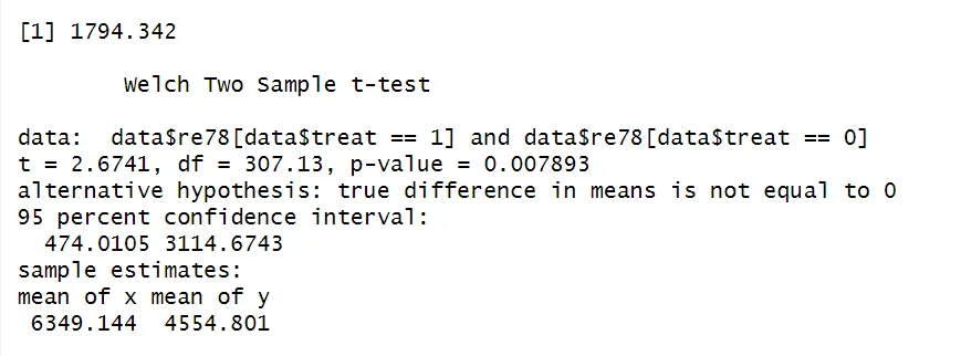
The difference-in-means estimate 1794.342 is returned. Additionally, a two-sample t-test compares the re78 values between the treatment and control group and tests the null hypothesis that the means of the two groups are equal. The p-value lower than 0.05 (here, 0.007) indicates the means are statistically significant different from each other.
Balance test
To check whether randomization went right and whether the treatment and control groups are balanced, we compare the observed covariates with a summary statistics table. The covariates of interest are defined by the columns_of_interest list. Then, the mean and standard deviation of each variable is calculated for both the treatment and control group, and t-tests are conducted to compare these means. The results are extracted and stored in vectors.
# Generate binary variable for unemployment
data$u74 = data$re74<0.0001
data$u75 = data$re75<0.0001

# Defining the covariates (columns) of interest
columns_of_interest = c("black","hispanic","age","married","nodegree","education","re74","re75")

# Calculate means and standard deviations
treatment_means = colMeans(data[data$treat==1,columns_of_interest])
control_means = colMeans(data[data$treat==0,columns_of_interest])
treatment_std = colSd(data[data$treat==1,columns_of_interest])
control_std = colSd(data[data$treat==0,columns_of_interest])

# Perform t-tests and extract results
t_test_results = sapply(columns_of_interest, function(x) {
  t.test(data[[x]][data$treat==1],data[[x]][data$treat==0])$statistic
})

t_test_pvalue = sapply(columns_of_interest, function(x) {
  t.test(data[[x]][data$treat==1],data[[x]][data$treat==0])$p.value
})

# Create summary table
df <- data.frame(
  Covariate = columns_of_interest,
  mean_control = round(control_means, digits = 2),
  sd_control = round(control_std, digits = 2),
  mean_treated = round(treatment_means, digits = 2),
  sd_treated = round(treatment_std, digits = 2),
  t_stat = round(t_test_results, digits = 1),
  p_value = round(t_test_pvalue, digits = 3)
)

kable(df)
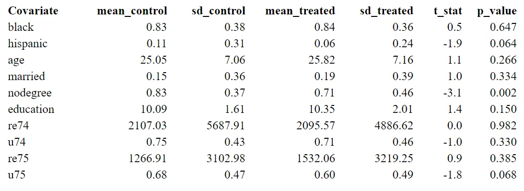
The first two columns present the results of the control group, and the third and fourth are the results of the treatment group.
Significant differences in some characteristics (p-value < 0.05) suggest an imbalance between the two groups. For example, since people with no degree are more likely to drop out of the treatment group, the amount of people with nodegree is significantly higher in the control group. If people with nodegree have lower earnings independent of whether they received a program, the treatment effect is likely to be overestimated. Matching offers a solution, where we can control for this kind of covariates.
Propensity score matching
To avoid the curse of dimensionality, since we have multiple observed covariates and relatively few observations, we use propensity score matching.
- Calculate the propensity score
Calculate the propensity score by estimating a logistic regression with the glm() function. The dependent variable is the treatment indicator, the independent variables include the covariates and interaction terms.
# Create interaction terms
data$re74nodegree = data$re74*data$nodegree
data$nodegreeeducation = data$nodegree*data$education
data$u75education = data$education*data$u75

# Run the logistic regression
propreg = glm(treat ~ re74 + u74 + re75 + u75 + nodegree + hispanic + education + nodegreeeducation + re74nodegree + u75education, family = binomial(link = "logit"),data=data)
summary(propreg)
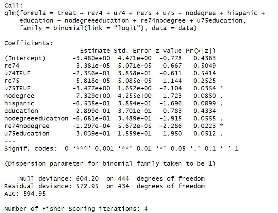
This logistic regression model estimates the propensity score, which is the probability of receiving the treatment given the observed covariates $\hat{P}(X_i)$.
Nearest neighbor propensity score matching
We now use the propensity scores to conduct nearest neighbor matching, ensuring balance between treatment and control groups. The matchit() function is used, in which the formula, the method (here, nearest) and the distance metric are specified. The distance metric is used to measure the similarity between individuals; it is calculated as the log odds ratio of the propensity score.
# Generate the matched data
match_prop <- matchit(treat ~ re74 +u74 + re75 + u75 + nodegree + hispanic + education + nodegreeeducation + re74nodegree + u75education, method = "nearest", distance = "glm", link = "logit", data=data )

# Data containing treated observations and their matched equivalence in the control group
data_match_prop <- match.data(match_prop)
Estimate the ATT by comparing the means of the outcome variable (re78) between the treated and control groups in the matched data.
# Estimate the ATT
mean_re78_match_prop <- aggregate(re78~treat,   data=data_match_prop, FUN=mean)

estimate_matching <- mean_re78_match_prop$re78[2]    -  mean_re78_match_prop$re78[1]

estimate_matching

# Another t-test to check if means are statistically different
t.test(data_match_prop$re78[data_match_prop$treat==1],data_match_prop$re78[data_match_prop$treat==0])
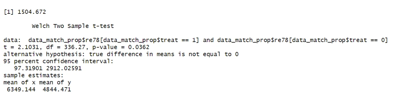
The difference between income is 1504, which is lower than the estimated ATT before matching. The p-value of 0.03 confirms the means are statistically different from each other.
This is in line with our reasoning: the treatment effect was underestimated when ignoring that on average the control group contained more people with nodegree, as a consequence of selective attrition.
SummaryApproximate matching, specifically Propensity Score Matching (PSM), addresses selection bias by matching individuals based on their propensity scores, representing the probability of receiving the treatment given observed covariates. This method helps mitigate the curse of dimensionality, where exact matching becomes impractical due to a large number of variables or continuous covariates.
Using a practical example from Imbens (2015) on the effect of job training programs on earnings, we demonstrated the application of PSM in R. By estimating propensity scores and conducting nearest-neighbor matching, we were able to assess the Average Treatment Effect on the Treated (ATT) and address potential bias from selective attrition, where people with no degree where more likely to drop out of the treatment group.