


Overview
Randomization is a fundamental principle in experimental design, aiming to have a good counterfactual and ensuring the treatment and control groups are similar except for being treated. However, in cases where treatment is not randomly assigned, confounding variables can bias the estimated causal effect.
Matching offers an alternative approach by basically creating an artificial counterfactual. This is done by pairing individuals or units based on specific observable characteristics to create comparable groups. This article provides a comprehensive introduction to matching, focusing on both the theory behind the method and practical applications.
Exact and approximate matching
Exact matching involves pairing individuals who share identical characteristics. This requires the observable characteristic on which pairing happens to be a binary variable. Also ideally, the control group has many observations at each distinct value of the binary variable the observations are matched on.
In contrast, approximate matching allows for some degree of flexibility and pairs on similar but not identical characteristics.
Identifying assumptions
 Summary
Two identifying assumptions should hold for exact matching to be valid:
-
Conditional Independence Assumption: Given observed covariates X, there are no systematic differences between treated and untreated units.
-
Overlapping support: Conditional on X, there are treated and untreated units.
1. Conditional Independence Assumption (CIA)
The Conditional Independence Assumption is the primary assumption underlying matching. It states that once we account for the observed characteristics of units or individuals, there should be no systematic differences in potential outcomes between the treatment and control groups.
Mathematically, this assumption is expressed as follows:
$(Y_{0}, Y_{1}) \perp T \:|\: X$
Where $Y_{0}$ and $Y_{1}$ are the potential outcomes in respectively the control and treatment group, which are independent of treatment assignment $T$ for each value of the observed covariates $X$. The $X$ is/are the binary variable(s) on which the observations are matched.
Important to note is that this assumption also implies no unobservable characteristics differing between the groups, impacting treatment likelihood or effects. When dividing the sample by $X$, for each value of $X$, the variation in $D$ is akin to random. In some cases, this condition is know to hold. A notable example is "Project STAR", where treatment was randoml assigned within schools but with varying likelihoods across different schools. Hence, school identity is included in $X$.
 Tip
TipWhile the absence of no unobservable characteristics cannot be directly tested, there are some methods to assess the plausibility of the assumption.
As discussed in Imbens (2015), one method is to calculate the causal effect of treatment on a pseudo-outcome that you know is unaffected by it, for example, a lagged outcome. If the treatment effect on the pseudo-outcome is close to zero, it strengthens the assumption's plausibility. Section VG (page 395) discusses this method in more detail.
2. Overlapping support
The assumption of overlapping support states that, conditional on observed covariates $X$, there exist both treated and untreated units across the entire range of $X$. In other words, there should be enough overlap in the distribution between the treatment and control groups to enable meaningful comparisons. This ensures that the treatment and control groups are comparable across all observed covariates, allowing for valid causal inference.
Exact matching estimator
If the above two assumptions are valid, the following identity follows:
$$ E[Y_1 - Y_0 | X] = \
E[Y_1 - Y_0 | X, D = 1] - E[Y_0 | X, D = 0] = \
E[Y | X, D=1] - E[Y | X, D=0] $$
Where: - $Y_1$ is the outcome for the treatment group - $Y_0$ is the outcome for the control group - $D$ is the treatment indicator (1 if treated, 0 if control)
The average effect of the treatment on the treated (ATT) is estimated by taking the expected outcome of the treatment group minus the expected outcome of the matched controls, averaged out over the treatment group.
The estimated average treatment effect on the treated ($\hat{d}_{\text{ATT}}$) is expressed as follows:
Where: - $N_{1}$ is the total number of units in the treatment group - $Y_{i}$ is the outcome variable of the treated unit $i$ - $Y_{j(i)}$ is the outcome variable of the control unit matched to unit $i$
TipThe counterfactual is the mean outcome in the control group for observations with the exact same characteristics.
Practical example
The most simple practical example of exact matching is given, with data simulated for this purpose. Say we are interested in finding the effect of a graduate traineeship program on earnings. We have data of 100 employees, of which 50 completed a traineeship at the start of their career (the treatment group) and 50 did not (the control group).
First, load the necessary packages, and the data set:

library(MatchIt)
library(ggplot2)
library(dplyr)

# Load data
data_url <- "https://raw.githubusercontent.com/tilburgsciencehub/website/master/content/topics/Analyze/causal-inference/matching/jobtraining_data.Rda"

data <- load(url(data_url))

View(data)
When observing the data, we notice the groups are not similar. The people in the treatment group, who followed the traineeship are on average younger (26 years) than the people in the control group (39 years):
# Average age for the treatment group
mean(data$Age[data$Treatment == 1])

# Average age for the control group
mean(data$Age[data$Treatment == 0])
The following histogram confirms this unequal distribution:
# Create a combined data frame for treatment and control groups
data$Group <- ifelse(data$Treatment == 1, "Treatment", "Control")

# Create the histogram
ggplot(data, aes(x = Age, fill = Group)) +
  geom_histogram(position = "identity",
                 alpha = 0.5,
                 bin_width = 1) +
  labs(title = "Age Distribution: Treatment vs. Control Group",
       x = "Age",
       y = "Frequency") +
  scale_fill_manual(values = c("blue", "red")
  )
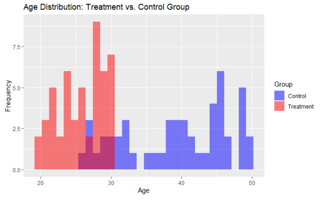
If younger people have lower earnings on average (which is likely to be the case), the effect of the traineeship is underestimated due to this unequal distribution of treatment assignment. First, we calculate the treatment effect while ignoring this potential bias:
ATT_original <-  mean(data$Earnings[data$Treatment == 1] - mean(data$Earnings[data$Treatment == 0]))

print(ATT_original)
The ATT is -998.26. So, not taking the average age difference into account, you find a negative effect of the traineeship program on earnings. The ATT is biased.
A solution is to match a treated employee to an untreated employee on age and compare their earnings instead. You can do this with the matchit function from the MatchIt in R, to match observations, specifying Treatment and Age.
matched_data <- matchit(Treatment ~ Age, data = data, method = "exact")

# Extract the matched dataset
matched_data <- match.data(matched_data)
Calculate the ATT, but now on the matched sample:
ATT_matching <- mean(matched_data$Earnings[matched_data$Treatment == 1] - matched_data$Earnings[matched_data$Treatment == 0])

print(ATT_matching)
The ATT is 7968.828, suggesting a positive effect of the traineeship program on earnings, which makes more sense!
OLS as a matching estimator
Another approach to control for the effects of other variables is to use Ordinary Least Squares (OLS) regression as a matching estimator. Regress the outcome variable ($Y$) on the treatment indicator ($D$), and the covariates ($X$).
furthermore, to understand how the treatment effect depends on observable characteristics $X$, we can include interaction terms between $D$ and $X$ in the regression model:
$Y = \beta_0 + \beta_1 D + \beta_2 * X + \beta_3 (D * X) + \epsilon_i$
Where - $Y$ is the outcome variable - $D$ is the treatment indicator (1 = treated, 0 = control) - $X$ is a vector of covariates - $D * X$ is the interaction effect between the treatment and covariate(s) X.
Effect coding
Effect coding is another approach to include these interaction terms, allowing for easier interpretation. It involves coding categorical variables such that the coefficients represent deviations from the overall mean. It can help understand how the treatment effect varies across different levels of X.
The regression equation with interaction terms included would look like this:
$Y = \beta_0 + \beta_1 D + \beta_2 * X + \beta_3 D * (X_i - \bar{X}) + \epsilon_i$
Where $D * (X_i - \bar{X})$ is the interaction between the treatment and the de-meaned covariate $X_{i} - \bar{X}$.
It captures how the treatment effect varies with deviations of the covariate $X$ from its mean value ($\bar{X}$). Specifically, $\beta_3$ indicates the additional effect of the treatment for each unit change in the covariate(s), compared to the average treatment effect.
When $X_i = \bar{X}$, the expected differences in outcomes is $\beta_2$. This is the ATE under conditional independence.
The ATT can be estimated as:
$\hat{\beta_2} + \frac{1}{N_1} \sum_{i=1}^{N_1} \cdot D_i \cdot (X_i - \bar{X}) \hat{\beta_3}$
The following R code creates a de-meaned variable for Age and runs the OLS regression with an interaction term between Treatment and Age_demeaned.
# Create a de-meaned covariate
data$Age_demeaned = data$Age - mean(data$Age)

# OLS regression with interaction term
ols_model <- lm(Earnings ~ Treatment * Age_demeaned, data = data)

summary(ols_model)
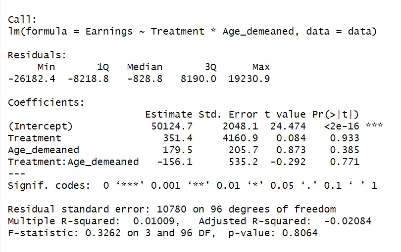
The coefficient for treatment is 351.4, indicating a positive but statistically insignificant effect of the program on earnings.
The estimate for the interaction term measures the dependence of the treatment effect on covariate Age. While insignificant, the negative sign indicates the effect of the program on earnings is reduced for individuals with an age that is further away from the mean.
TipFor a full interpretation of the summary output of the regression model, refer to this topic.
OLS versus Matching method
While using OLS regression and adding covariates for each observable characteristic, and the Matching method both rely on the Conditional Independence Assumption to facilitate causal inference, opting for matching has its advantages. Reasons to consider matching instead of the OLS method are outlined in the table below:
| ------------------------------------- | ------------------------- | ----------------------------- |
| Functional form | Linear functional form not required | Assumes linear functional form |
| Comparable untreated units | Identifies whether there are comparable untreated units available for each treated unit. | Does not identify whether there is a lack of comparable untreated units for each treated unit. |
| Counterfactual weighting | Expected counterfactual for each treated unit weighted based on observable characteristics of the untreated units. | Uses whole control group for determining the expected counterfactual. |
SummaryThe identifying assumptions Conditional Independence and Overlapping Support are crucial. When these assumptions hold, matching provides a framework for establishing causal relationships in observational studies. An example of exact matching is given, where individuals were paired based on the identical values of their age.
In OLS regression, incorporating an interaction term between the treatment indicator and the (de-meaned) covariate allows for assessing how the treatment effect varies across different levels of the covariate.
You can continue the content of matching by reading the next topic on Approximate Matching.