Overview

Take advantage of the versatility of containerized apps on Docker and the power of Google Cloud to easily reproduce and collaborate on projects!

This building block is meant to be a step-by-step guide in order for you to learn:

• How to reproduce a containerized project environment on a Google Cloud virtual machine.
• How to run Jupyter Notebook in your cloned environment and how to access it so you can interact with the project’s Python code.

Warning

Good to know!

This building block complements our previous one on how to export project environments with Docker. Thus, while the steps here presented are valid in a general sense, their details were designed to match the particularities of the containerization process described in that building block. We strongly recommend you to visit it to get a more comprehensive understanding of the present one’s content and the containerization process.

Tip

Not using Virtual Machines?

Cloud virtual machines offer many advantages in terms of flexibility and computational power.

However, if you are trying to replicate a Docker-containerized project environment in your local computer, simply follow Steps 2 and 3 of this building block and access Jupyter Notebook as you usually do.

Alternatively, after Steps 2 and 3, you can jump straight to Step 5 and follow it employing your internal IP address (Which is typically: 127.0.0.1) instead of the cloud virtual machine’s external IP.

Step 1: Install and Set up Docker in your Google cloud instance

Google Cloud’s virtual machines are configured to operate on Debian Linux by default. As a result, installing Docker on these machines follows the standard procedure for Linux-based systems. You can learn how to do so by visiting our building block on how to set up Docker, which covers the setup of Docker in Windows, MacOS, and Ubuntu Linux.

If you prefer to cut to the chase, we have condensed these instructions into two Docker installation scripts available below. These scripts work for Debian and Ubuntu Linux, which are among the most commonly used Linux distributions on Google Cloud’s virtual machines.

Feel free to either follow these scripts step-by-step or save them in a shell script format file (.sh) to then upload and execute them on your virtual machine. Either method will successfully install Docker on your VM and thus allow you to continue with the building block.

Warning

Not working?

Docker’s setup process differs slightly across Linux distributions, so make sure to follow the appropriate instructions for your distribution whether it is Ubuntu, Debian, or any other. If your Google Cloud VM is not running in any of these distributions, check the official Docker documentation which provides guidelines for installing Docker in many different Linux distributions.

After completing the Docker setup steps outlined above, you’ll need to prefix all Docker commands with sudo when running them on your VM. If you find it more convenient to bypass this requirement, you can run the following code snippet:

# Add your user to the `docker` command group
# to get rid of the need to `sudo` to handle Docker

$ usermod -aG docker your-user-name

$ newgrp docker

Step 2: Build the environment’s image from a Dockerfile

After successfully installing Docker, the next step is to build your project’s dockerfile. This file provides Docker with the instructions needed to create a Docker image.

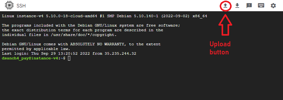
To start, you’ll need to transfer your project’s dockerfile to your virtual machine. If you’re using Google Cloud’s browser-based SSH interface, the simplest way to do this is by clicking the ‘Upload file’ button, located near the top right corner of the screen. From there, you can select and upload the dockerfile from your local machine, and it will be transferred to your virtual machine instance.

Tip

Work smart, not hard

If the image of the project environment you are trying to import has been published on Docker Hub, you don’t need to upload and build it manually as described.

Instead you can use the docker pull command and Docker will automatically retrieve and build the image from Docker Hub. Then you will be ready to jump to Step 3.

Upon having uploaded the dockerfile, navigate to the directory where it is located and run the following code snippet to instruct Docker to build the environment’s image from it:

# Build a Docker image 
$ docker build .

You can think of the Docker image as a template of our environment, and the dockerfile as the manual with instructions on how to build this template.

This template can be used to generate containers, which can be thought of as individual instances based on the template. So, each time you tell Docker to generate a new container from the image, it generates a brand new copy of the environment from the template you previously provided.

Warning

Do not forget to include the dot at the end of the code block above as it indicates to Docker that it has to look for your dockerfile in the current directory.

With this command, Docker will build the image alongside its context, the latter comprised of all the files located in the same path as your dockerfile and which are relevant to the image. In the context of a research project whose environment is being reproduced with Docker, this would generally imply that you should place all the files which are relevant to your project’s environments in the same directory as the dockerfile.

Tip

A good practice

You can assign a name (i.e. tag) to your new Docker image by adding to the code above the flag -t followed by the name you want to assign in between the build command and the dot at the end as shown in the code block below.

Don’t worry if you don’t include this information, as in that case, Docker will automatically assign a name to the image. However, specifying a name is advisable as it will allow you to identify your images more easily.

You can view a list of all your docker images in your Docker Desktop dashboard or by typing docker images in the command line.

# Build a Docker image and assign a name to it
$ docker build -t <your-image-name> .

Step 3: Docker compose

Docker compose is a tool within the Docker ecosystem whose main functionality is to coordinate your containers and provide them with the services required to run smoothly and in the intended manner.

These services include actions such as communication between containers or starting up containers that require additional instructions to do so. Although this can sound a bit confusing if you are new to Docker (you can learn more about Docker compose here), the key takeaway is that it will assist and simplify the task of replicating your environment by providing some extra information to Docker about how to do so. Particularly, in this context, the docker-compose file will be in charge of the following two “services”:

1. Connect your environment’s container with the rest of your system to make it possible to move files from one to the other.
2. Launch Jupyter Notebook.

Warning

Docker-compose files must be YAML files, so make sure that your docker-compose file is denoted as such with the extension .yml.

Upload your docker-compose.yml in the same way you did it with your dockerfile, navigate to the directory where it is located and then execute the following:

# Build the docker image
$ docker compose up 

Tip

An advantage of Docker Hub

If your environment’s dockerfile is hosted on Docker Hub you don’t need to manually build it as explained in Step 2 of this building block.

Instead, you could just run its associated docker-compose file as shown above and Docker will take care of the rest automatically, pulling the image from Dockerhub, building it, and finally executing the instructions included in the docker-compose itself.

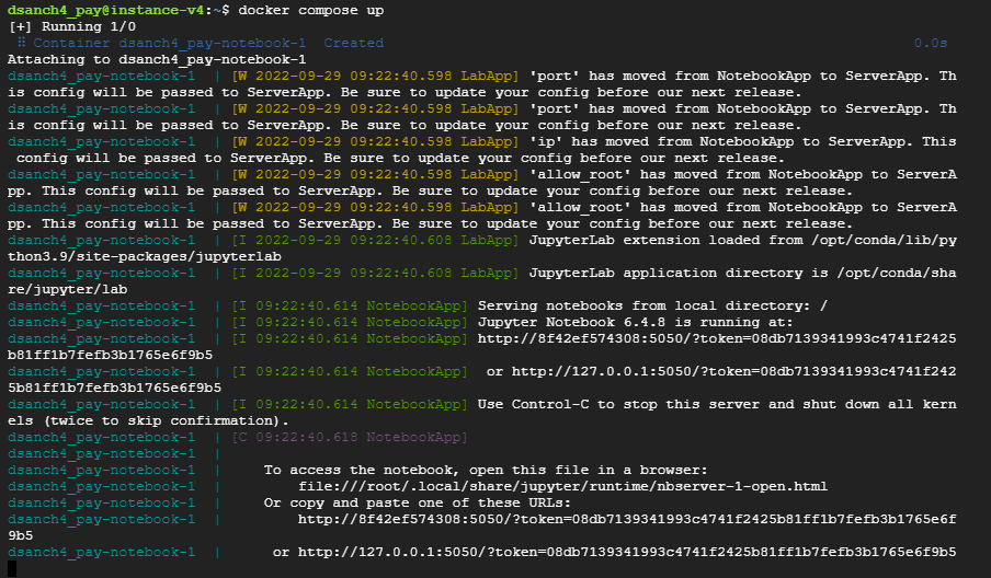
If the execution of docker-compose was successful that means that your environment’s container is up and with Jupyter Notebook running. In such case you should see something in your command line resembling the following:

Step 4: Expose the port where Jupyter Notebook is running

At this point, you need to make the Jupyter Notebook running on your container accessible from the outside. The first element we need for this task is to know in which port of your instance is it running.

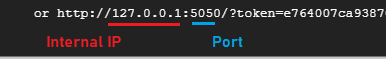
To know this we just have to take a closer look at the last line of the output shown in the command line after having executed docker compose up. At the beginning of the line, you should see an address like the one shown below, from there you are interested in the four digits underlined in blue coming after the internal IP and before the slash. These correspond with the port where Jupyter Notebook is running in your instance.

Warning

Make sure

Note that the port in which your container’s Jupyter notebook is running (i.e. the four-digit number that corresponds to that underlined in blue in the previous image) will probably be different from the one shown in the image above.

Tip

It is possible to adjust the port in which you want Jupyter Notebook to be executed. In the context of this building block, this is defined by the instructions contained in the environment’s docker-compose. Learn more about docker-compose.

Now, you should go back to the Google cloud console and click the button “Set up firewall rules” which is below your instances list. Then click again on the “Create firewall rule” option located towards the upper side of the screen. There you have to:

1. Add a name of your choice for the rule (e.g. Jupyter_access_rule)
2. Make sure that traffic direction is set on “Ingress”
3. Indicate to which of your instances you want this rule to apply by selecting “Specified target tags” in the “Targets” drop-down list, and then specify the names of these in the “Target tags” box below. Alternatively, you can select the option “All instances in the network” in the drop-down menu so the rule automatically applies to all your instances.
4. Introduce “0.0.0.0/0” in the field “Source IPv4 ranges”
5. In the section “Protocols and ports” check “TCP” and then in the box below introduce the four-digit number that identifies the port where Jupyter Notebook is being executed in your instance.

Warning

Safety first

In point 3 of the steps listed above you are told to introduce “0.0.0.0/0” in the field “Source IPv4 ranges”. Beware this means that your instance will allow connections from any external IP (i.e. any other computer). If you are concerned about the safety risk this involves and/or you know beforehand the list of IP addresses that you want to allow to connect to your instance, you could list them here instead of typing the one-size-fits-all “0.0.0.0/0”.

After completing the fields as described, you can go to the bottom and click on “create” to make the firewall rule effective.

Step 5: Access Jupyter Notebook within your environment’s container

To finally access the Jupyter Notebook running inside your environment’s container you have to go back to the Google Cloud console list of virtual machine instances and copy your instance’s external IP direction.

With this information, you can open a web browser on your local computer and type the following in the URL bar:

http://< external_ip_address >:< jupyter_port >

Example

Imagine the external IP of your instance is “12.345.678.9” and the port where Jupyter is running is port “1234”. In that case, you should paste the following URL into your browser: http://12.345.678.9:1234

After introducing the URL as indicated, you will be directed to your instance’s Jupyter Notebook landing page. Here Jupyter will request you a token to grant you access. This token can be found in the same output line of your Google Cloud instance’s command line where you look at the port where Jupyter is being run.

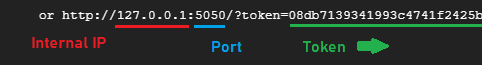
As you can see in the image above, the token consists of a string of alphanumeric characters comprising all that comes after the equal sign ("=").

Warning

Note that in the image above the token is not fully depicted. You must copy all the characters that come after the equal sign, which compose a character string that is noticeably larger than the one underlined in green.

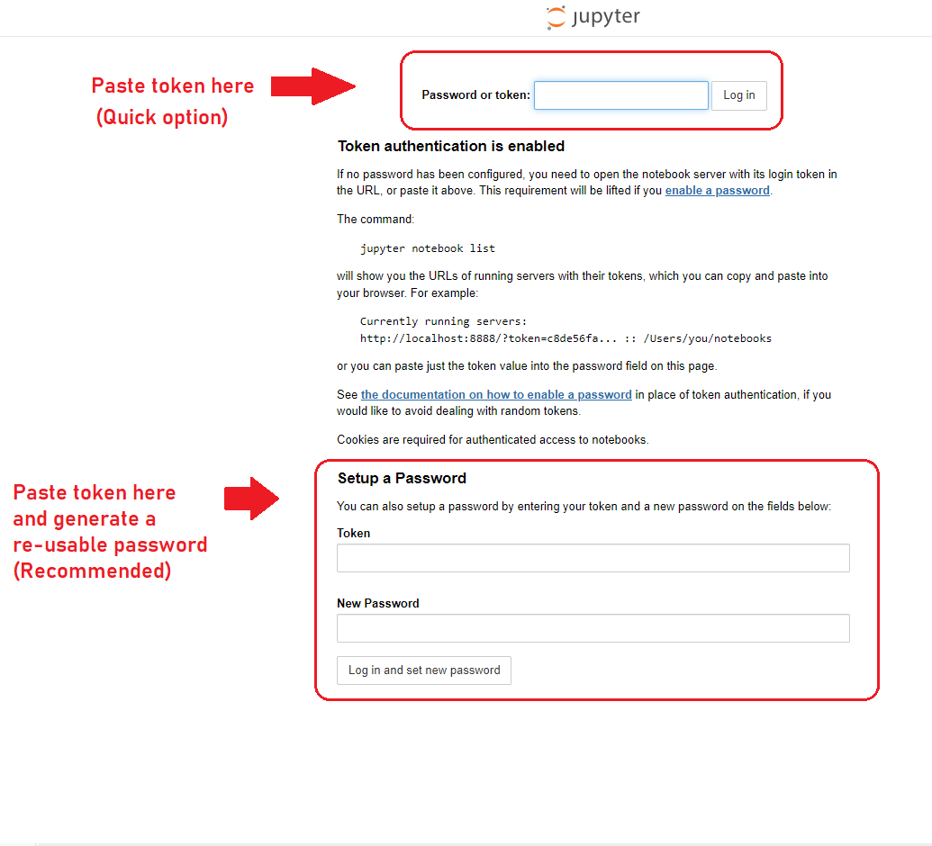
Now simply introduce this token in the box at the top of the landing page and click on “Log in” to access your environment.

You can also paste your token in the “Token” box at the bottom of the page and generate a password with it by creating a new password in the “New Password” box.

This way the next time you revisit your environment you will not need the full token, instead, you will be able to log in using your password. This is particularly useful in case you lose access to your token or this is not available to you at the moment.

Summary

By the end of this building block, you should be able to:

• Initialize and Deploy Jupyter Notebook in Docker: Set up a Docker environment and deploy a Jupyter Notebook using Docker Compose within a Google Cloud VM instance.

• Identify and Expose Jupyter Notebook’s Port: Locate the specific port where the Jupyter Notebook is running and configure the Google Cloud firewall settings to expose this port safely, facilitating external access.

• Access and Secure Your Jupyter Notebook: Access the Jupyter Notebook remotely through a web browser using the VM’s external IP address and port, and understand how to secure the environment using tokens or a password.

Additional Resources

• Learn how to Configure a VM with GPUs in Google Cloud.
• Cheat-sheat on Docker Commands