


Introduction
To illustrate the theory of Fuzzy RDD, we use the example given by Cattaneo, Idrobo & Titiunik (2023) in their paper on Extensions of Regression Discontinuity. A study by Londono-Velez, Rodriguez, and Sanchez (2020) investigates the effects of governmental subsidy for post-secondary education in Colombia. The subsidy is only offered if students meet a fixed set of requirements: obtaining a certain test score and having a certain household wealth index. Since the eligibility is based on whether observed scores meet the fixed cutoffs, this is an example of a regression discontinuity design.
As some students that were eligible did not receive the subsidy, it means that this is a Fuzzy RDD. Although in this study there are two conditions to be met so that the treatment (subsidy) is received, which makes this a multi-dimensional regression discontinuity design, we treat it as a one-dimensional RDD by only taking the students whose test score is above the cutoff. Hence, the only running variable remains the household wealth index, with the treatment being the receipt of the subsidy.
Descriptive Statistics
The dataset used by Cattaneo, Idrobo & Titiunik (2023) contains 23,132 observations of students whose test score is above the cutoff and whose household received welfare benefits. We identify the following elements:
- running variable $X$: the difference between a student's wealth index and the corresponding cutoff
- treatment assignment $T$: indicator that equals 1 when the running variable $X < 0$, indicating that the student is eligible to receive the subsidy
- treatment received $D$: indicator that equals 1 when the student actually receives the treatment
- outcome of interest $Y$: indicator that equals 1 if the student enrolled in a higher education institution after receiving the treatment
In the dataset, 66.7\% of students are eligible for the treatment, but only 40\% actually receive it.
Fuzzy RD in Practice
To investigate the intention-to-treat effects of assigning the subsidy, we first need to analyze the first stage relationship between the eligibility to receive the funding ($T$) and the actual receipt ($D$). Below we show the corresponding RD plot with default choices, as described in RD plots.
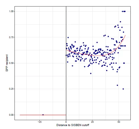
The plot shows that the example has one-sided non-compliance, meaning that no student whose test score is under the cutoff receives funding, but some students whose scores are above the cutoff fail to receive funding, although they are eligible. The red line is the estimated probability of receiving the treatment and it jumps from 0 to approximately 0.60 at the cutoff.
We can use the rdrobust function to estimate the first stage relationship between subsidy eligibility and the receipt of funding ($D$).

out <- rdrobust(D, X1)
summary(out)
Output:
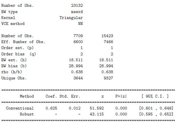
The shown coefficient of 0.625 represents the first-stage effect, which corresponds to the jump seen in the graph above. The effect is highly significant, showing that around 62\% of those who are barely eligible to receive subsidy actually receive it.
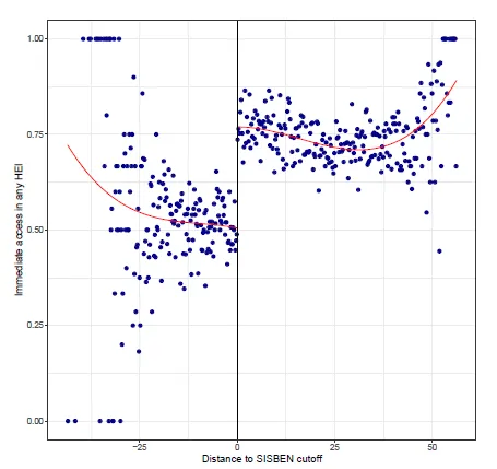
Next we analyze the effect of the ITT on the outcome of attending post-secondary education after becoming eligible ($Y$). For this we use a third-order polynomial fit to avoid overfitting near the boundary. Below is the corresponding plot.
To code this we use the same function, but change the parameter from D to Y.
out <- rdrobust(Y, X1)
summary(out)
Output:
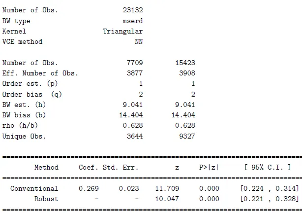
The output shows that around 27\% (0.269) of students whose scores are above the cutoff are more likely to enroll in post-secondary education, jumping from around 50\% enrollment below the cutoff to around 77\% above the cutoff, as visible in the graph.
In Fuzzy RDD, we defined the formula for the Fuzzy RD parameter: $\tau_{FRD} = \tau_{Y}/\tau_{D}$
Thus, we can calculate $\tau_{FRD}$ by taking the ratio $0.269/0.625 = 0.4304$. This means that receiving the subsidy results in a 43\% increase in the probability of enrolling in post-secondary education for students who are compliers.
 Summary
In this topic, a practical, hands-on example of the Fuzzy RDD methodology is explored.
In the next topic in the series on regression discontinuity, the local randomization approach is explained, that augments the traditional continuity-based RD design by considering the running variable as quasi-randomized within a specific bandwidth surrounding the cutoff.