


Overview
In the realm of machine learning, two primary branches are supervised and unsupervised learning. Supervised learning consists both regression, which predicts continuous values, and classification, where the model endeavors to assign correct labels to input data. Our focus in this article lies within the domain of classification. Through practical examples and Python implementations, we'll navigate the essentials of classification, including how models are trained on datasets and evaluated to ensure their efficacy before making predictions on new, unseen data.
Classification
In the classification process, a classifier learns to map input vectors to specific classes or labels by training on numerous examples of input-output pairs. These pairs, also known as predictor-target samples.
In classification tasks, the range of possible labels is usually constrained, typically determined by the number of distinct classes under consideration. The number of classes influences whether we employ binary or multi-class classifiers, impacting factors such as the choice of cost function and evaluation metrics.
To illustrate these concepts, we will use the Digits dataset, a well-known dataset consisting 1,797 images of handwritten digits, each annotated with a numerical label ranging from 0 to 9.
Let's download the dataset using Scikit-Learn.

from sklearn.datasets import load_digits

# Load the Digits dataset
digits = load_digits()

# assign X and y to predictors and target
X = digits.data
y = digits.target
Before diving into training process, it's important to familiarize ourselves with the data it contains. Running the following code snippets give a basic overview of the dataset's contents.
# get the description of digits dataset
print(print(digits.DESCR))
Now you know that X contains 64 variables, with each pixel representing one variable. Let's visualize one of the numbers.
import matplotlib.pyplot as plt

sample = X[1001]

# Plot the sample
plt.imshow(sample.reshape(8, 8), cmap='gray')  #each sample is a 8x8 image
plt.axis('off')
plt.show()

# print the label attached to the sample
print(y[1001])
Before training a model on a dataset, it's crucial to prepare the data to ensure its compatibility with the model. You can learn about the necessary steps in the article titled Linear Regression for Prediction in Python.
Binary Classification
Binary classification is the process of distinguishing between only two classes. The output of a binary classifier is typically a binary decision, such as "yes" or "no", "spam" or "not spam", "positive" or "negative", etc. Common example of binary classification tasks are email spam detection, Medical diagnosis, Fraud detection, and so on.
We apply binary classification by classifying digit 5 vs other digits. There are several classifiers can be effective for our case. One commonly used algorithm is the Decision Tree classifier. It is known for ability to handle high-dimensional data efficiently and effectively, making them suitable for image classification tasks like Digits dataset.
from sklearn.model_selection import train_test_split
from sklearn.tree import DecisionTreeClassifier
from sklearn.metrics import accuracy_score

# Classify digit 5 versus not digit 5
binary_y = (y == 5).astype(int) # To have a binary classification problem

# Split the dataset into training and testing sets
X_train, X_test, y_train, y_test = train_test_split(X, binary_y, test_size=0.2, random_state=42)

# Initialize the Decision Tree classifier
DT = DecisionTreeClassifier(random_state=42)

# Train the classifier
DT.fit(X_train, y_train)

# Make predictions on the testing set
y_pred = DT.predict(X_test)

# Calculate accuracy
accuracy = accuracy_score(y_test, y_pred)
print("Accuracy:", accuracy)
performance measure of Binary classifier
Accuracy may not provide a good assessment of performance, particularly when dealing with imbalanced datasets where one class dominates the others. For instance, in the Digits dataset, only 10% of the instances are labeled as 5. This means that if we simply predict non-fives for all images, we could achieve an accuracy of 90%. Therefore, we use precision, recall, and F1-score as alternative performance measures to provide a more comprehensive evaluation.
Precision measures the portion of correctly predicted positive instances out of all instances predicted as positive.
Recall measures the portion of positive samples are predicted as positive.
F1-score is calculated by taking harmonic mean of precision and recall.
-
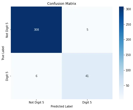
The confusion matrix visualizes the model's performance by showing the counts of true positives, false positives, true negatives, and false negatives. With these counts, you can compute precision, recall, accuracy, and the F1-score.
# import required liblaries
from sklearn.metrics import f1_score, confusion_matrix, precision_score, recall_score
import seaborn as sns
import matplotlib.pyplot as plt

# calculate precision
precision = precision_score(y_test, y_pred, average='weighted')
print("Precision:", precision)

# Calculate recall
recall = recall_score(y_test, y_pred, average='weighted')
print("Recall:", recall)

# Calculate F1-score
f1 = f1_score(y_test, y_pred)
print("F1-score:", f1)

# Compute the confusion matrix
conf_matrix = confusion_matrix(y_test, y_pred)

# Display the confusion matrix
plt.figure(figsize=(8, 6))
sns.heatmap(conf_matrix, annot=True, cmap="Blues", fmt="d", xticklabels=["Not Digit 5", "Digit 5"], yticklabels=["Not Digit 5", "Digit 5"])
plt.xlabel("Predicted Label")
plt.ylabel("True Label")
plt.title("Confusion Matrix")
plt.show()
Above code snippest gives this confusion matrix. It reveals that 41 samples of digit 5 are correctly predicted, while 6 samples of digit 5 are erroneously classified. Within this context, 41 represents true positives, whereas 6 corresponds to false negatives. Furthermore, the matrix indicates 308 true negatives and 5 false positives.
Multi-Class Classification
Multi-classifiers are used to distinguish more than two classes. For example, in image classification, each image can belong to one class among more than two classe. There are three strategies commonly employed for performing multiclassification.
1- The One-vs-All classifier, also known as the One-vs-Rest classifier, is a technique used for multi-class classification tasks. For instance, in the case of classifying 10 digits, we train 10 binary classifiers, each dedicated to distinguishe one digit from the rest.
To assign a class to an image, we obtain the decision score from each classifier for that image. Then, we select the class associated with the classifier that outputs the highest score.
Advantages: Since each class is uniquely represented by its own classifier, analyzing the classifier associated with a specific class offers insights into that class. This approach is the default choice by most of the classifiers in Sklearn library.
# Split the dataset into training and testing sets
X_train, X_test, y_train, y_test = train_test_split(X, y, test_size=0.2, random_state=42)

# Initialize the classifier
clf = DecisionTreeClassifier(random_state=42)

# Train the classifier
clf.fit(X_train, y_train)

# Make predictions on the testing set
y_pred = clf.predict(X_test)

# Calculate accuracy
accuracy = accuracy_score(y_test, y_pred)
print("Accuracy:", accuracy)
2- The One-vs-One classifier creates separate classifiers for every pair of classes. When making predictions, the class with the most votes from all classifiers is selected.
Advantage: While slower than the "one-vs-all" approach due to its $O(n_{\text{classes}}^2)$ complexity (which results in 45 classifiers for the Digits dataset), the "one-vs-one" method requires each classifier to be trained on a subset of the dataset containing only two labels.
You can adopt the above code to implement multiclassification using One-vs-One
# import OneVsOneClassifier
from sklearn.multiclass import OneVsOneClassifier

# Initialize the classifier
ovo_clf = OneVsOneClassifier(clf)

# Train the classifier
ovo_clf.fit(X_train, y_train)

# predictions on the testing set
y_pred = ovo_clf.predict(X_test)

# Calculate accuracy
accuracy = accuracy_score(y_test, y_pred)
print("Accuracy:", accuracy)
3- In the case of multiclassification, some algorithms like Random Forest is capable of directly classifying instances without the need for intermediary binary classification steps.
# import RandomForest Classifier
from sklearn.ensemble import RandomForestClassifier

# Initialize the classifier
rf_clf = RandomForestClassifier(n_estimators=100, random_state=42)

# Train the classifier
rf_clf.fit(X_train, y_train)

# predictions on the testing set
y_pred = rf_clf.predict(X_test)

# Calculate accuracy
accuracy = accuracy_score(y_test, y_pred)
print("Accuracy:", accuracy)
In this approach, you can obtain the probabilities of assigning each image to each class. The following code do this task.
# Get the probabilities assigned to each image for each class
probabilities = rf_clf.predict_proba(X_test)

# Display the shape of the probabilities array
print("Shape of probabilities array:", probabilities.shape)

# display the matrix of probaability of each image belonging to eachh class
probabilities
 Tip
TipCommon algorithms used for multiclassification are K-nearest neighbor, Decision Tree, Random Forest, Gradient Boosting, and Naive Bayes.
Performance measures in multiclassification
Running the code for performance evaluation in binary classification can also be used for multiclassification tasks.
In multiclassification scenarios, the size of each axis of the confusion matrix corresponds to the number of classes. For instance, when classifying the Digits dataset, the confusion matrix is a square matrix with dimensions $10 \times 10$. Each row represents the true class labels, while each column represents the predicted class labels.
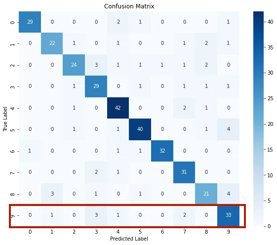
As an Example, the confusion matrix reveals that the digit 9 was correctly predicted for 33 images, while it was incorectly predicted as 7 twice, as 4 once, as 3 thrice, and as 1 once.
 Summary
- An introduction to classification
- Applying classification on Digits Dataset to classify handwriten images
- Binary classification by Decision Tree algorithm
- performance measure of Binary classification
- Multi classification approaches:
- One-vs-All classification
- One-vs-One classification
- Classification by probability distribution
- Performance measures in multi-classification problems