


Overview
Rmarkdown serves as an helpful tool for generating reproducible reports, academic papers, and technical documents using the programming language R and the writing language markdown.
This article focuses on figure presentation in Rmarkdown. It discusses chunk options, standardizing global figure settings, and employing LaTeX. Additionally, it discusses how to save the created figures to specified directories for organized file management.
For a practical application of these techniques, a downloadable Rmarkdown file is available allowing for direct engagement with the discussed formatting approaches.


# Download the Rmarkdown file by clicking the top right button
Formatting through Chunk Options
RMarkdown enables figures to be directly formatted via chunk options. This allows for full control over the presentation of figures within your report.
Here is a list of figure formatting options:
fig.align: Adjust the alignment of your figure.- Options include "default", "center", "left", or "right".
fig.cap: Allows you to provide a caption for your figure, input as a character vector:- For instance, "A detailed caption here".
fig.height&fig.width: Specify the dimensions of your figure in inches.- each argument takes one number (e.g., 7, or 9_).
out.height&out.width: Adjust the size of the figure in the output document, useful for scaling figures.- For
LaTeXoutputs, use dimensions like".12\linewidth"or "10cm"; - For
HTML, use "300px".
- For
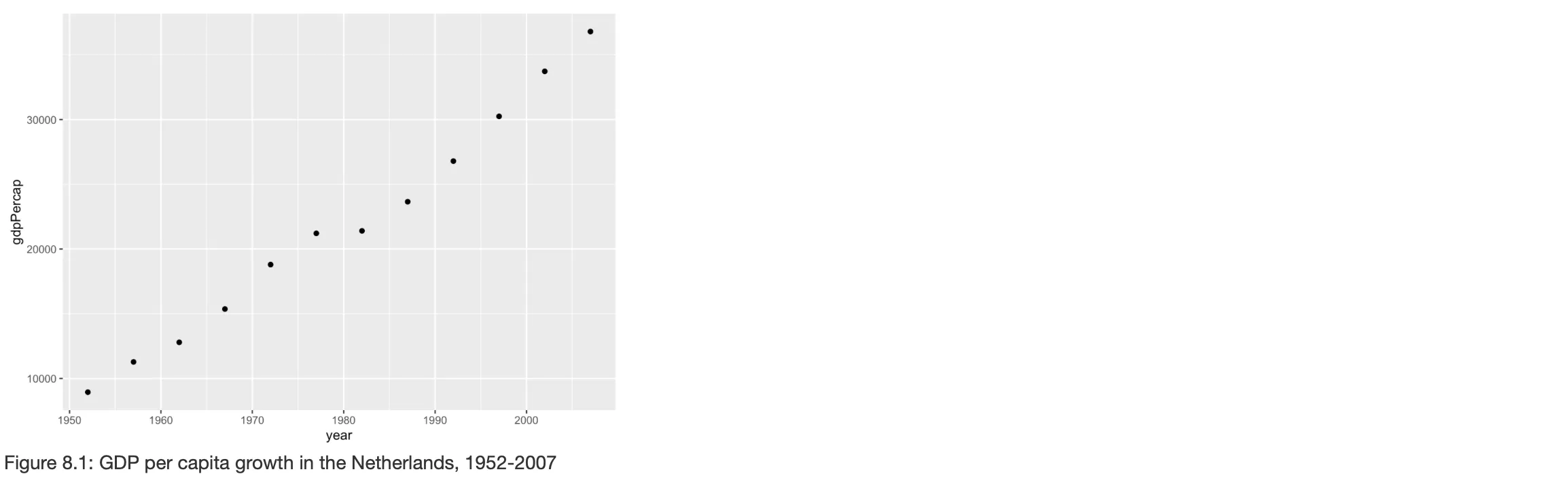
Here's an example of how to use these options in a code chunk:
# Code Chunk specification
{r example-figure, # Code Chunk Key
    fig.cap="GDP per capita growth in the Netherlands, 1952-2007",
    fig.width=7,
    fig.height=5,
    fig.align="left",
    out.width="50%"}

# Code
library(ggplot2)
library(dplyr)
library(gapminder)

gapminder %>%
  filter(country == "Netherlands") %>%
  ggplot(aes(x = year, y = gdpPercap)) +
  geom_point()
And it will look like this:
Global Settings for Figure Formatting
To maintain consistency across all figures within your figure and avoid specifying the formatting process each code chunk seperately, global figure settings can be specified at the start of the document. This applies uniform appearance for all figures, saving time and ensuring aesthetic coherence.
You can do this with the following code:
knitr::opts_chunk$set(fig.width = "Your Settings", fig.height = "Your Settings", fig.align='Your Settings', out.width = "Your Settings")
Saving Figures
Adjusting the display properties of figures can change their presentation within the document, but it doesn't automatically save them as separate files. For figures to be saved, you must modify the YAML header to include keep_md: true, as shown below:
---
output:
  html_document, pdf_document, word_document, or any other format:
    keep_md: true
---
This setup generates folders like "YOURFILENAME_files" to store figures. To directly control where your figures are saved, use the fig.path option in a setup chunk at the start of your document. Setting fig.path tells RMarkdown the exact folder to store your figures. For example, to save all figures in a folder named "figs", add this to a code chunk within your document:
knitr::opts_chunk$set(fig.path = "figs")
 Tip
TipThis approach will save your figures directly to the current working directory. However, if you wish to specify a different location, you can redefine your working directory using the setwd() function. A better approach is to utilize relative paths for organizing your output more effectively. For example, you can save figures to a specific folder by specifying a path like "../gen/output/figs". This approach helps in keeping your project's file structure organized and accessible.
Using Latex for Formatting
Step 1: Specify extra_dependencies: "subfig" in your YAML
For a more coherent organization and presentation in your document, consider using the subfig package in LaTeX. This package can be used to arrange multiple sub-figures within a singular figure environment. In addition, it allows for each sub-figure to have its own individual caption. This capability is particularly beneficial for comparative analyses or presenting grouped data in a cohesive manner.
To incorporate sub-figures into your Rmarkdown document include the subfig package in your document's YAML via the extra_dependencies option as shown below:
---
output:
  "Your Output Format":
    extra_dependencies: "subfig"
---
 Warning
Use tabs, not spaces, for indentation in Rmarkdown to avoid rendering issues.
Step 2: Adjust Code Chunk Options
To construct a single figure with multiple sub-figures, place all related plots within a single R code chunk. Thereafter, you can adjust the code chunk options, as discussed earlier in the article, to control the layout and captioning.
Here are some specific commands to use with the subfig package:
- Main Caption: Use the
fig.capoption to provide a general caption for the entire figure. - Sub-figure Captions: Use
fig.subcapfor individual sub-figure captions.- Supply a character vector for the captions, such as
c('(1)', '(2)', '(3)'), corresponding to each sub-figure.
- Supply a character vector for the captions, such as
- Figure Arrangement: Control the arrangement of your figures in columns with
fig.ncol.- By default, all plots are arranged in a single row.
- Plot Size: Manage the size of each plot with the
out.widthoption.- Standard practice is to calculate the width as 100% divided by the number of columns, ensuring all plots have equal width and fit within the page margins properly.
For example, to align three sub-figures into two columns with equal width and centered alignment, your syntax in the R code chunk might look as follows:
# Code chunk specification
{r, fig.cap='Figure about LaTeX sub-figures', fig.subcap=c('(1)', '(2)', '(3)'), fig.ncol=2, out.width="50%", fig.align="center"}

# Your R code for the sub-figures
plot(1:10)
boxplot(Sepal.Width ~ Species, data = iris)
hist(rnorm(100))
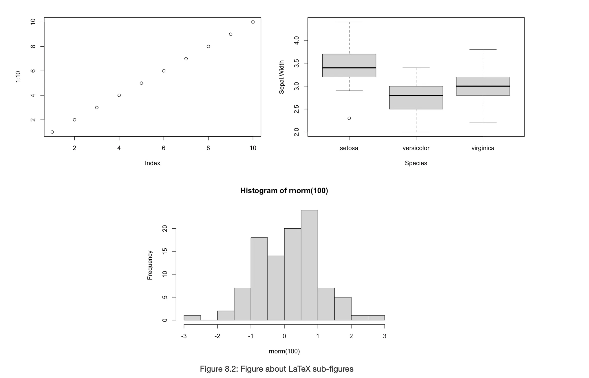
This setup sets the basis for your sub-figures to be neatly organized, each with its own caption, within a single, well-captioned figure.
TipHow to dynamically cross-reference figures generated by code chunks within your Rmarkdown document, please check the explanations provided in a related article.
 Summary
This article provides an overview of using Rmarkdown for academic writing, focusing on figure management, figure organization, and formatting techniques.
- Figure Formatting: through chunk options and global settings, including alignment, dimensions, and captions, to ensure a consistent presentation in your
Rmarkdowndocument. - Figure Saving: Automates the saving of figures and specifies their storage locations, facilitating organized and efficient document management.
_LaTeXFormatting_: EmploysLaTeXto create sub-figures within a single figure environment, enabling comparative analyses and cohesive presentation of grouped data.