


Overview
Rmarkdown is a format designed for creating reproducible and dynamic reports using R.
In this article, we explore how to convert regression models into LaTeX-formatted equations using the equatiomatic package, a time-saving approach compared to the error-prone task of manually typing equations.
This article covers practical examples, including handling categorical variables, interaction terms, and customizing the LaTeX equation outputs. This approach eases and automates the process of adding equations into Rmarkdown reports.


# Download the Rmarkdown file by clicking the top right button
Transforming Regression Models into LaTeX Equations
When conducting statistical data analysis, it is often necessary to incorporate regression models into a report. Common models in R, such as lm() and glm(), are not automatically formatted for direct inclusion in reports. In academic texts, such as books, journal articles, and reports, you usually encounter neatly written equations like:
$y = \alpha + \beta_1 \cdot x1 + \beta_2 \cdot x2 + \epsilon$
This equation needs to be manually specified in your Rmarkdown document as follows:
_y = \alpha + \beta_1 \cdot x1 + \beta_2 \cdot x2 + \epsilon
Manually transcribing these structured equations can be prone to errors, especially as the complexity of the model increases.
The equatiomatic package bridges the gap between the raw outputs of these models and their formatted equation counterparts. It
eases the process by automating the conversion of statistical model outputs, generated by functions like lm(), into LaTeX equations. This makes them suitable for integration into RMarkdown documents.
Let's explore the package capabilities with practical examples.
Practical Steps for Model Equation Extraction
Step 1: Initial Setup, Installing and Loading equatiomatic
Begin by installing the equatiomatic package using the commands below:
# To install the equatiomatic package, you have two options:
# For the latest development version, install from GitHub:
remotes::install_github("datalorax/equatiomatic")
# For the stable version, install directly from CRAN:
install.packages("equatiomatic")

# After installation, load the package into your R session:
library(equatiomatic)
Step 2 Model Fitting
Now, fit a regression model using for example the lm() function:
# Fit your model:
fit <- lm(mpg ~ cyl + disp, mtcars)
Step 3: Equation Extraction
Finally, use extract_eq() to display your model as a LaTeX equation:
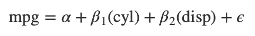
# Display the theoretical model as an equation
equatiomatic::extract_eq(fit)

 Tip
TipTo display only your equation without showing the code, set echo = FALSE in the code chunk. This will keep your article tidier.
Complex Model Considerations
While the basic model described above might be quickly typed out by those familiar with LaTeX syntax, the real strength of the outlined process becomes evident when dealing with models that include categorical variables with multiple levels and interactions. These elements introduce complexity not only to the model's output but also to the manual transcription of the equation.
Categorical Variables
Equatiomatic automates the inclusion of categorical variables into LaTeX-formatted equations. It recognizes and incorporates the levels of categorical variables as subscripted elements within the equation.
fit_cat <- lm(Sepal.Length ~ Species, iris)
extract_eq(fit_cat)

Interaction terms
The package also supports the conversion of interaction terms to LaTeX formatted equations.
fit_int <- lm(data = iris, Sepal.Length ~ Species * Petal.Length)
extract_eq(fit_int)

Customize Equation Ouput
The automation provided by the method above greatly simplifies equation generation. However, tailoring these equations to meet specific documentation requirements often necessitates further adjustments. The equatiomatic package offers a set of options for customizing equations.
Syntax
To improve the readability and precision in your documentation, equatiomatic provides several syntax customization options:
- Coefficients Customization:
_use_coefs_: Opt to display actual coefficient values instead of Greek symbols. By default, this is set to FALSE._terms_per_line_: This controls the number of terms displayed on each line of the equation._wrap_: Adjusts the equation width to fit within your document's margins.
- Variable Presentation:
- By default, variable names appear in plain text. For italics, which might be preferred for mathematical variables, set
ital_vars = TRUE.
- By default, variable names appear in plain text. For italics, which might be preferred for mathematical variables, set
- Intercept Notation:
- Change the default notation from alpha (𝛼) to beta (𝛽₀) for the intercept by setting
intercept = "beta".
- Change the default notation from alpha (𝛼) to beta (𝛽₀) for the intercept by setting
Advanced Custom Syntax with Raw TeX:
While "alpha" and "beta" are the options for the intercept argument, The raw_tex and greek parameters offer the flexibility to define custom syntax for both the intercept and coefficients. For instance:
extract_eq(,
  wrap = TRUE,
  intercept = "\\hat{\\tau}",
  greek = "\\hat{\\gamma}",
  raw_tex = TRUE
)
Practical Examples
Beyond simple regression models, equatiomatic accomodates more types of models.
library(palmerpenguins)
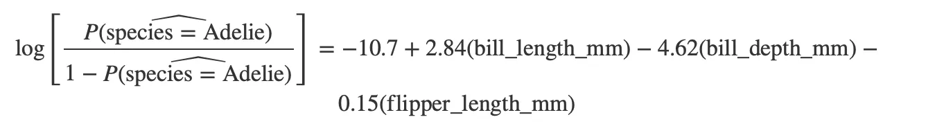
fit_glm <- glm(species ~ bill_length_mm + bill_depth_mm + flipper_length_mm, data = penguins, family = binomial)
extract_eq(fit_glm, use_coefs = TRUE, terms_per_line = 3, wrap = 80)
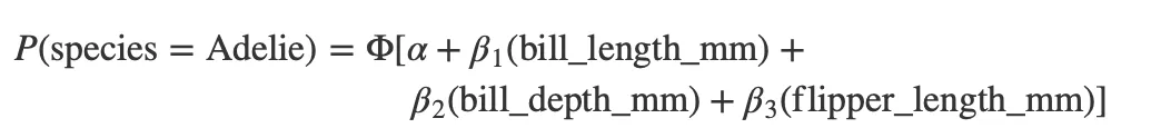
fit_probit <- glm(species ~ bill_length_mm + bill_depth_mm + flipper_length_mm, data = penguins, family = binomial(link = "probit"))
extract_eq(fit_probit, use_coefs = FALSE, terms_per_line = 2, wrap = 40)
 Warning
The equatiomatic package does not yet support mathematical functions (e.g., log, exp, sqrt) or models like polynomial regressions and multi-level (mixed effects) models.
 Summary
This article introduces equatiomatic for converting regression models into LaTeX-formatted equations, easing the presentation of statistical analyses in RMarkdown. It discusses practical examples, customization options, and the package's capability to handle both simple and complex models, underscoring its potential value in academic documentation.