


Overview
In this building block, you will learn the essential steps of text pre-processing in R. You will use the 'tm' package and create a corpus, the main structure for managing text documents, to then conduct a range of text preprocessing tasks. These steps will allow you to transform raw text into a more structured and suitable form for analysis. Finally, you will explore the process of visualizing and analyzing text data using term-document matrices and word clouds.
Introduction
Text mining is all about deriving insights from unstructured text data such as social media posts, consumer reviews, and newspaper articles. The ultimate goal is to turn a large collection of texts, a corpus, into insights that reveal important and interesting patterns in the data. This could include either computing the sentiment of a text or inferring the topic of a text among other common tasks.
Before we can move into the analysis of text, the unstructured nature of the data means there is a need to pre-process the raw text to transform it to provide some additional structure and clean the text to make it more amenable for further analysis. To illustrate some common pre-processing steps we will take some data on Amazon reviews and use the tm package in R to clean up the review texts.
In the GitHub repository linked below you can find the full R script text_cleaning.R which is used as a reference during this building block. We will cover the most relevant code snippets within it. However, we strongly recommend that you review the full script and keep it on hand while following the building block so you can replicate the presented results and get a comprehensive picture of the content.
Steps for pre-processing text data
Install tm package

install.packages("tm")
library(tm)
Step 1: Create Corpus
The tm package uses a so-called corpus as the main structure for managing text documents. A corpus is a collection of documents and is classified into two types based on how the corpus is stored:
- Volatile corpus (VCorpus) - a temporary R object. This is the default implementation when creating a corpus.
- Permanent corpus (PCorpus) - a permanent object that can be stored outside of R (e.g., in a database)
Next, to create the corpus you need to identify the source type of the object. Sources abstract input locations, like a directory, a connection, or simply an R vector, to acquire content uniformly.

- DataframeSource - for data frame structures like CSV files
- DirSource - for file directories
- VectorSource - for a vector of characters interpreting each component as a document
These three are the most widely used source types.
Now, let’s create our corpus!
review_corpus<- VCorpus(DataframeSource(kindle_reviews))
# the review text is stored under dataframe 'kindle_reviews'
 Tip
TipA data frame source interprets each row of the data frame x as a document. The first column must be named "doc_id" and contain a unique string identifier for each document. The second column must be named "text" and contain a UTF-8 encoded string representing the document's content. Optional additional columns are used as document-level metadata.
Step 2: Cleaning Raw Data
The tm package has several built-in transformation functions that enable pre-processing without too much code!
This procedure might include (depending on the data) :
- The removal of extra spaces
- Lowering case
- The removal of special characters
- The removal of URLs and HTML tags
- The removal of stopwords
Lowering case
Lowering case is helpful to reduce the dimensions by decreasing the size of the vocabulary and is weighed similarly when counting the frequency of words.
review_corpus<- tm_map(review_corpus, content_transformer(tolower))
Whitespaces, Punctuation and Numbers
Whitespaces, while ensuring readability, can introduce inconsistencies in text data, necessitating standardized handling. Punctuation, essential for sentence structure, can cause variability in text mining, making its removal or normalization crucial. While numbers offer context, they might divert attention from the main textual content, so their normalization or removal can be beneficial.
review_corpus<- tm_map(review_corpus, stripWhitespace) # removes whitespaces
review_corpus<- tm_map(review_corpus, removePunctuation) # removes punctuations
review_corpus<- tm_map(review_corpus, removeNumbers) # removes numbers
Special characters, URLs or HTML tags
For this purpose, you may create a custom function based on your needs and use it neatly under the tm framework.
# create custom function to remove other misc characters
text_preprocessing<- function(x) {
    gsub('http\\S+\\s*','',x) # remove URLs
    gsub('#\\S+','',x) # remove hashtags
    gsub('[[:cntrl:]]','',x) # remove controls and special characters
    gsub("^[[:space:]]*","",x) # remove leading whitespaces
    gsub("[[:space:]]*$","",x) # remove trailing whitespaces
    gsub(' +', ' ', x) # remove extra whitespaces
  }

# Now apply this function
review_corpus<-tm_map(review_corpus,text_preprocessing)
Stopwords
Stopwords such as “the”, “an” etc. do not provide much of valuable information and can be removed from the text. Based on the context, you could also create custom stopwords list and remove them.
review_corpus<- tm_map(review_corpus, removeWords, stopwords("english"))
# OR: creating and using custom stopwords in addition
mystopwords<- c(stopwords("english"),"book","people")
review_corpus<- tm_map(review_corpus, removeWords, mystopwords)
Step 3: Tokenization, Stemming and Lemmatization
The process of splitting text into smaller bites called tokens is called tokenization. Each token can then be used as an input into a machine learning algorithm as a feature. Furthermore, the two techniques to normalize tokens are stemming and lemmatization.
-
Stemming: it is the process of getting the root form (stem) of the word by removing and replacing suffixes. However, watch out for overstemming or understemming. - Overstemming occurs when words are over-truncated which might distort or strip the meaning of the word.
E.g., the words “university” and “universe” may be reduced to “univers” but this implies both words mean the same which is incorrect. - *Understemming occurs when two words are stemmed from the same root that is not of different stems.* E.g., consider the words “data” and “datum” which have “dat” as the stem. Reducing the words to “dat” and “datu”, respectively, results in understemming. -
Lemmatization: is the process of identifying the correct base forms of words using lexical knowledge bases. This overcomes the challenge of stemming where words might lose meaning and makes words more interpretable.
In this example we will stick to Lemmatization, which can be conducted in R as shown in the code block below:
# Lemmatization
review_corpus<- tm_map(review_corpus, content_transformer(lemmatize_strings))

# Note: `lemmatize_words` function is used when you have a vector of words but in a corpus we do not have a vector of words. Instead, we have strings with each string being a document's content. Hence, we use `lemmatize_strings` function instead.
Step 4: Creating the Term-Document Matrix
The corpus can now be represented in the form of a Term-Document Matrix, which represents document vectors in matrix format. The rows of this matrix correspond to the terms in the document, columns represent the documents in the corpus and cells correspond to the weights of the terms.
tdm<- TermDocumentMatrix(review_corpus, control = list(wordlengths = c(1,Inf)))
Inspect and Analyze your Textual Data
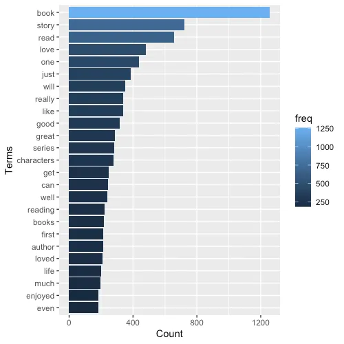
Inspecting Word Frequemcies
Now that we've created the term-document matrix, we can start analyzing our data. For example, imagine you want to quickly view the terms with certain frequency, say at least 50. You can use findFreqTerms() for this. findAssocs() is another useful function if you want to find associations with at least certain percentage of correlation for certain term.
# inspect frequent words
freq_terms<- findFreqTerms(tdm, lowfreq=50)

term_freq<- rowSums(as.matrix(tdm))
term_freq<- subset(term_freq, term_freq>=20)
df<- data.frame(term = names(term_freq), freq = term_freq)
# Now plotting the top 25 frequent words
library(ggplot2)

df_plot<- df %>%
  top_n(25)

# Plot word frequency
ggplot(df_plot, aes(x = reorder(term, +freq), y = freq, fill = freq)) + geom_bar(stat = "identity")+ scale_colour_gradientn(colors = terrain.colors(10))+ xlab("Terms")+ ylab("Count")+coord_flip()
TipTerm-document matrices tend to get very big with increasing sparsity. You can remove sparse terms, i.e., terms occurring only in very few documents. This reduces the matrix dimensionality without losing too much important information. Use the removeSparseTerms() function for this.
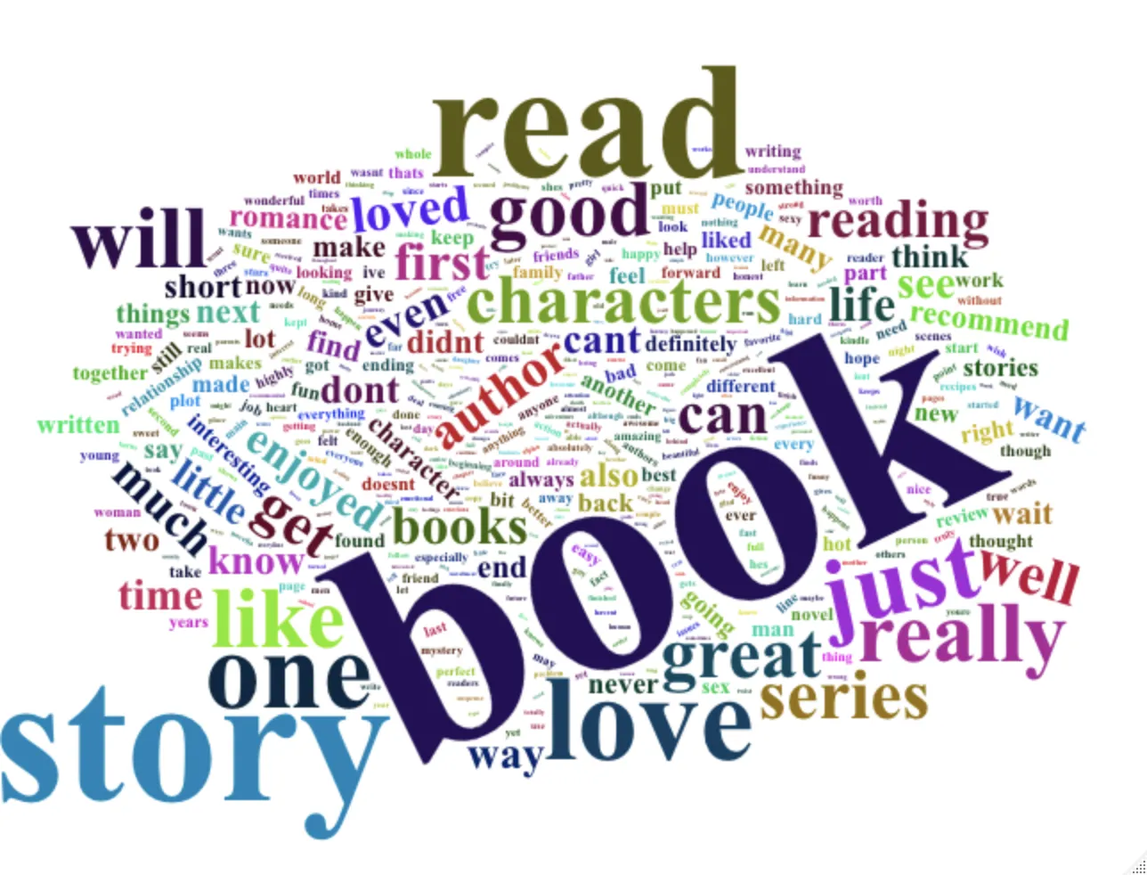
Visualizing the Data
Let’s build a word cloud that gives quick insights into the most frequently occurring words across documents at a glance. We will use the wordcloud2 package for this purpose.
install.packages("wordcloud2")
library(wordcloud2)

# calculate the frequency of words as sort by frequency
wordcloud2(df, color = "random-dark", backgroundColor = "white")
That's it! You're now equipped with the basics in doing text analysis using the tm package in R!
 Summary
- Text mining extracts insights from unstructured text data and the main goal is to transform a corpus of texts into interpretable patterns and valuable insights.
-
Steps to Pre-processing raw text data:
- Lowercase: Normalize text by converting it to lowercase.
- Remove special characters, punctuation, and numbers.
- Eliminate URLs, HTML tags, and other unwanted elements.
- Strip extra whitespaces and standardize formatting.
- Remove common stopwords that add little meaning.
- Stemming: reduces words to their root form by removing suffixes.
- Lemmatization: identifies base forms based on lexical knowledge.
-
Term Document Matrix (TDM): Represent the corpus as a matrix of terms and documents. Each row is a term, each column is a document, cells hold term weights.
-
Visualise the processed text data using Word Clouds which provide a quick overview of frequent words.
Tip