


Overview
Parallel computing significantly accelerates computations by dividing tasks into smaller segments, which are then processed concurrently across your computer's cores. While certain libraries in R, like data.table and dplyr, already support parallel processing, researchers can also adapt non-parallel code for concurrent execution.
This article introduces the fundamentals of parallel computing through straightforward R code examples, focusing on two methods: the multicore and socket approaches.
 Warning
The multicore method is not compatible with all operating systems. It works on Unix-like systems such as macOS and Linux, but not on Windows. However, since Google Colab operates on Linux, it can facilitate multicore parallelization on any system. The socket approach is universally compatible.
How Does Parallelization Work?
The Central Processing Unit (CPU) contains units called "cores," which determine the number of tasks your computer can perform simultaneously. Creating clusters of cores allows you to assign different parts of a task to each cluster. In theory, the more cores you have, the faster you can process computations—potentially reducing the time by the number of available cores. However, overhead costs such as subprocess initiation and data duplication generally limit these theoretical time savings. We will explore this further in the concluding section of this article.
To find out how many cores you can utilize simultaneously, use the detectCores() function in R.

# Load the 'parallel' package
library(parallel)

detectCores()
The Multicore Approach
A straightforward implementation of the multicore approach is the mclapply() function from R's parallel package. While apply() iterates over data structures, applying a function to each element, mclapply() enhances this by executing the iterations across multiple processes (i.e., cores). This method replicates the entire current R session onto each core, making it unnecessary to re-export variables or reload packages.
Example
Consider calculating the average sepal length for each species in the iris dataset within R. To get familiar with the dataset, you might start by running summary(iris).
 Tip
TipThis Google Colab file includes all the code examples from this article!
# Load necessary packages and the Iris dataset
library(dplyr)
library(datasets)
data(iris)

# Define the function
calculate_mean_sepal_length <- function(df) {
  species <- unique(df$Species)
  means <- vector("numeric", length(species))
  for (i in 1:length(species)) {
    Sys.sleep(2)  # Simulates a 2-second computation delay
    means[i] <- mean(df[df$Species == species[i], "Sepal.Length"])
  }
  return(data.frame(Species = species, Mean_Sepal_Length = means))
}
The function introduces a computational delay of 2 seconds per iteration to simulate an intensive task. We will compare the execution times between standard and parallel processing using the system.time() function.
# Normal execution (sequential)
start_time_normal <- Sys.time()
result_normal <- calculate_mean_sepal_length(iris)
end_time_normal <- Sys.time()

time_normal <- end_time_normal - start_time_normal
The result (result_normal) is as follows:
| Species | Mean_Sepal_Length | |
|---|---|---|
| 1 | setosa | 5.006 |
| 2 | versicolor | 5.936 |
| 3 | virginica | 6.588 |
Now, let's apply parallel processing using mclapply():
# Parallel execution using mclapply
start_time_multi <- Sys.time()

result_multi <- bind_rows(
  mclapply(
    split(iris, iris$Species), calculate_mean_sepal_length
  )
)
end_time_multi <- Sys.time()

time_multi <- end_time_multi - start_time_multi
Compare the execution times:
time_normal
time_multi
Parallel processing shows a marked improvement, reducing the execution time from 6.018 seconds to 4.035 seconds. Note that these times may vary based on your system's hardware.
The Socket Approach
The socket approach differs from the multicore method by requiring you to manually create a cluster and distribute the code and data across its nodes. This results in additional overhead compared to the multicore method, where such exports are unnecessary. However, this way of parallelization gives you more control over what data and code your cores will be exposed to.
Example
To illustrate, we'll detail how to establish a cluster and execute tasks in parallel.
WarningEach core will run a separate instance of R in the socket approach. If your system prompts you to allow R to accept incoming connections, you should approve it.
- Identify Available Cores
Start by determining the number of cores your system can utilize.
# Determine the available number of cores
ncpu <- detectCores()
The number of cores varies by system; in this example, it is 2 on the Google Colab Notebook that we used to develop this article. You might want to use less than 100% of your cores to save some CPU capacity for other tasks.
- Create a Cluster
Next, use the makePSOCKcluster() function to specify the number of cores for your cluster based on the previously determined value.
# Create a parallel cluster
cl <- makePSOCKcluster(ncpu)
- Parallel Execution
Since the socket approach starts with a clean slate, you must explicitly transfer any required packages, variables, or functions to each cluster node using the clusterExport() function.
# Ensure necessary packages are loaded
library(parallel)
library(dplyr)

# Export the required function to the cluster
clusterExport(cl, 'calculate_mean_sepal_length')

# Define the parallel computation function
calculate_mean_sepal_length_parallel <- function(df) {
  clusterApplyLB(cl, split(df, df$Species), calculate_mean_sepal_length)
}

# Execute the parallel computation
start_time_socket <- Sys.time()
result_socket <- bind_rows(
  calculate_mean_sepal_length_parallel(iris)
)
end_time_socket <- Sys.time()
time_socket <- end_time_socket - start_time_socket
The result_socket dataset will display the mean sepal length for each species, similar to result_normal.
TipConsider using the parLapply() function to leverage the lapply() functionality across multiple cores in a socket cluster.
- Time Comparison
Finally, compare the execution times to assess the efficiency of parallel processing.
time_normal
time_socket
Again, the parallelized task was quicker, taking 4.035 seconds with the socket approach versus 6.018 seconds for the standard method.
When to Parallelize?
As mentioned earlier, achieving the ideal theoretical time savings is rare due to the overhead associated with executing code and combining results from multiple cores. Additionally, parallel processing often requires duplicating large datasets across all cores, which can lead to capacity issues. Moreover, there are development costs involved in adapting code for parallel execution, and some researchers may find it cumbersome to manage complex parallel code.
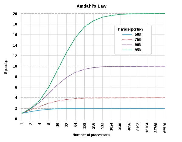
Despite these challenges, it is often worthwhile to consider parallelization, especially when code needs to be executed repeatedly, such as in reproducible research pipelines. A key concept to understand in this context is Amdahl's Law, which posits that the potential speedup of a task is limited by the number of cores available and the proportion of the task that can be parallelized. This principle is depicted in the following graph from Wikipedia:
The table below, based on Josh Errickson's article, summarizes the key differences between the multicore and socket approaches.
| Multicore | Socket |
|---|---|
| Available on Unix-like systems, e.g., macOS and Linux. Can also use Google Colab. | Compatible with all systems, including Windows. |
| Generally faster due to less overhead. | Slower because it requires launching new R instances on each core. |
| Does not require re-exporting variables or reloading packages. | Requires separate exports of variables, packages, etc., to each process. |
| Simpler to implement. | More complex due to additional setup requirements. |
WarningAs each core essentially starts a "new" R session, generating random numbers in parallel may be problematic. The parallel package, however, offers solutions to ensure reproducibility across cores (see Chapter 20.4 of this guide for details).
 Summary
Parallelization offers significant advantages, particularly for extensive computations. By distributing work across multiple cores, it not only speeds up processing times but also helps to prevent memory runtime errors. However, not all tasks are suited for parallel processing, and sometimes, the overhead can outweigh the benefits. With this foundation, you can now explore the potential of parallel computing in your own projects!