Introduction
Statistical power is an important but often overlooked concept in statistical and econometric analysis. Broadly, it refers to how likely we are to detect an effect if there is one. Imagine that you are looking for certain information in a document written in a foreign language. The better your understanding of that foreign language (higher statistical power), the more likely you'll be to find the information that you need. Conversely, if your understanding of the language is poor (low statistical power), you'll be less likely to find the information even though it is in the document.
More formally, statistical power can be defined as the probability of rejecting the null hypothesis when the alternative hypothesis is true. In this sense, it is closely related to the concept of type II error, i.e., failing to reject a false null hypothesis (also known as a false negative or error of omission). Indeed, statistical power = 1 – prob(type II error).
What does this mean in practice? Let’s say we are studying the relationship between enrolling in a skill training programme and future earnings. We assume that there is an effect of the programme on earnings: therefore, our null hypothesis of no effect is false, and the alternative hypothesis is true. Statistical power gives us the probability that we do in fact find an effect of the programme on earnings. For example, if our power is 0.6, there is a 60% chance that we find a statistically significant treatment effect. Similarly, there is a 40% chance of incurring in type II error, that is, not finding a statistically significant effect even though there is one. So, if we ran this estimation 100 times, without changing any of its properties (e.g., sample size or the hypothesised effect size), we would expect to obtain a statistically significant effect 60 times.
Because statistical power depends on sample size, it is especially relevant in the context of randomised experiments, where we can, to some extent at least, choose sample size ourselves. In such settings, we can conduct a power analysis to find the minimum sample size we need to have a certain level of power. Usually, this level is set at 0.8, although some practitioners recommend setting it higher, at 0.9.
The importance of statistical power
Why is low statistical power problematic? Firstly, because it means that we are less likely to detect an effect if there is one. This reduces our ability to evaluate policies and treatments. If we can only find a certain effect 20% of the time, for instance, it is more likely that we find no effect even though there is an effect in reality. This could lead to us to discard useful treatments or to fail to detect harmful effects of certain interventions.
Secondly, low power means that if we do find an effect, it’s more likely that it is exaggerated or even false. If we have a power of 0.2, we correctly detect an effect (reject the null) 20% of the time. This 20% includes the most extreme cases of the treatment having an effect (i.e., the highest 20% of the distribution of effect sizes). Therefore, any effects we find with a power of 0.2 will be in the highest quintile of effect sizes. Smaller effect sizes, which are more likely in reality (they occur 80% of the time), will simply be discarded as statistically insignificant. Thus, if we find an effect, we will only be seeing the strongest possible effects and will overestimate the true average effect size, which lies somewhere in those 80% which we fail to detect.
In summary, studies with low power are not only less likely to detect true effects, but will also exaggerate the sizes of any effects they detect. Therefore, whenever we can somehow influence statistical power, especially in experimental settings, we should ensure that our study has as much power as possible given budget and time constraints. As previously mentioned, the typical ‘golden standard’ is to have a power of at least 0.8.
Increasing statistical power
So how can we influence the power of our study and ensure it meets the established criteria? We can do so by changing one or more of the four variables which determine statistical power:
-
Sample size: a larger sample size increases power. Small sample sizes reduce the precision of comparisons between the treatment and control groups, and therefore make it more difficult to find a statistically significant effect, which reduces power.
-
Significance level ($\alpha$): the significance level can be seen as our standard for rejecting the null hypothesis, or, equivalently, for accepting that there is a statistically significant effect. The stricter our standard for rejecting the null (lower $\alpha$), the less likely it is that we reject it (i.e. the less likely that we find a statistically significant effect), so a lower $\alpha$ reduces power.
-
Hypothesised effect size: this is the smallest difference in means between the treatment and control groups that we want to be able to detect as statistically significant. For this reason, this parameter is also often known as the minimum detectable effect. Naturally, the larger the difference between the treatment and control groups, the more likely it is that we obtain a statistically significant effect. Therefore, a larger effect size increases power.
-
Variation in the outcome: this measures noise in the outcome variable. The more noise there is, the more difficult it is to extract a statistically significant treatment effect from that noise. Hence, more variation in the outcome reduces power. In practice, variation in the outcome is usually captured by the standard deviation of the outcome.
Warning
In observational studies, an additional variable of relevance is variation in treatment exposure. However, as this building block focuses mostly on experimental settings, its role is not discussed here.
Thus, we can increase power by increasing sample size, increasing the significance level, increasing our expected effect size, or reducing variation in the outcome. Increasing the significance level is generally not an option, because we want to keep type I error (the false positive rate; i.e. how likely we are to reject the null when there is no effect – when the null is true) low, usually at the 5% level ($\alpha$ = 0.05). Therefore, we are left with three options:
-
Increasing the sample size. This just means including more subjects in our study. Doing this is the most straightforward way of increasing power.
-
Increasing the expected effect size. This can be done by intensifying the treatment intensity or ‘dose’ and maximising treatment take-up in the treatment group. This way, we attempt to widen the difference in outcome means between the treatment and control groups. And if we expect this difference to be larger, it is also reasonable to aim for a larger minimum detectable effect.
Tip
Ensuring that treatment is delivered in sufficient doses and to as many subjects as possible in the treatment group is part of improving treatment fidelity. Treatment fidelity refers to the extent to which the treatment is delivered competently and as intended by the researcher.
-
Reducing variation/noise in the outcome. We can reduce noise by improving the quality of our outcome measures (minimising measurement error) and minimising heterogeneity in the characteristics of the subjects in our study. Additionally, we can measure the outcome at multiple points in time in the post-treatment period and compute an average. This can allow us to remove noise originating from seasonality, measurement error, and time-specific idiosyncratic shocks.
Power Analysis
The advantage of experimental studies is that we can to some extent control the above parameters. This also means that experimental researchers are expected to ensure that their studies have sufficient power. A typical way of doing this is conducting power analysis before designing our study. The goal of power analysis is to determine the minimum sample size we need to obtain a sufficient power (given the minimum detectable effect size, outcome noise, and the significance level) or to determine what minimum detectable effect size we can aim for (given sample size, outcome noise, and the significance level).
Power analysis can be done analytically or by simulation. The latter case is more relevant for observational studies, whereas the analytical approach is convenient for experiments. The formula for minimum sample size for a given level of power is the following:
$n = 2(z(\alpha) + z(1-\beta))^2\frac{s^2}{d^2}$
Where $z(x)$ is the z-score of $x$, $\alpha$ is the significance level, $\beta$ is the type II error rate (so $1-\beta$ is power), $s$ is the standard deviation of the outcome variable and $d$ is the minimum detectable effect size. If we are interested in computing $d$ given $n$ instead, we can easily rearrange for $d$.
In most settings, we use 0.05 as our significance level and 0.8 as our desired power. Setting $\alpha = 0.05$ and $\beta = 0.2$, we can derive the following rule of thumb for sample size calculations:
$n = 2(z(0.05) + z(0.8))^2\frac{s^2}{d^2}$
$n = 2(1.96 + 0.84)^2\frac{s^2}{d^2}$
$n = 15.6\frac{s^2}{d^2}$
Which is often simplified to just:
$n \approx 16\frac{s^2}{d^2}$
Using this formula, we could calculate the sample size manually. However, it is of course more practical to do so in R. For this, we can use the 'pwrss' package.
 Tip
TipThere are other packages that also calculate power in R, for example 'pwr' or 'retrodesign', which is also used to compute size and magnitude errors.
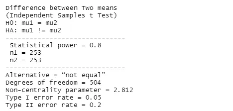
First, we use power analysis to calculate the minimum sample size. We use 0.05 as our $\alpha$ and 0.8 as our desired power, and we are looking for a standardised (i.e., relative to the standard deviation of the outcome variable; also known as Cohen's d) minimum effect size of 0.25 (a quarter of a standard deviation).
Output:

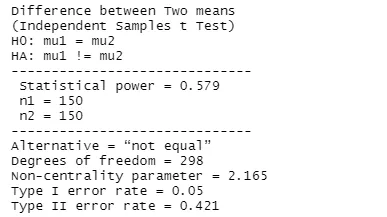
We see that to obtain a power of 0.8 and detect an effect of at least 0.25, we need 253 subjects in the treatment and control groups each. Now, suppose that we already have a certain sample size and want to find out what the power of our study would be if we used that sample size. Assume we have a sample size of 150 in each group and aim to detect an effect of 0.25, as previously.
Output:

As can be seen in the output, if we use a sample size of 150 in each group and want to identify an effect of at least 0.25, our study has a power of around 0.58. This means that the false negative rate is 42%, i.e., assuming there is an effect, we will not be able to detect it 42% of the time.
Summary
Statistical power is an important but often disregarded concept in empirical research. It allows us to gain insight into the credibility of our results: low-powered studies are less likely to be able to detect an effect if there is one and any effects they do detect are likely to be exaggerated or anomalous. Power analysis also allows us to calculate what sample size we would need in an experimental study in order to attain a certain level of power, typically 0.8.
Statistical power depends positively on sample size, the minimum effect size we are looking for, and on the significance level $\alpha$ and negatively on noise in the outcome variable. Therefore, in order to increase power, we can increase sample size or the minimum detectable effect size, or reduce variation/noise in the outcome.


