


Overview
Heteroskedasticity is a common issue cross sectional, time series and panel data analysis. And refers to the failure of the homoskedasticity assumption when the variance of the error terms varies across observations in a regression model. This inconsistency can skew the standard errors, undermining the validity of statistical inferences derived from Ordinary Least Squares (OLS) regressions.
This article explores methods for detecting and correcting heteroskedasticity using R, including both graphical and statistical tests, and discusses approaches to correct for heteroskedasticity.
Underneath we have a straightforward example of heteroskedasticity to help you become familiar with the concept:
 Example
Consider the regression equation, that models the relationship between income and expenditure on meals:
$Y_i = \beta_0 + \beta_1 X_i + \epsilon_{i}$
Where: $Y_i$ represents the expenditure on meals for the i-th individual, $X_i$ is the income and $\epsilon_{i}$ is the error term associated with each observation.
Heteroskedasticity Interpretation
As an individual's income increases, the variability in their meal expenditures also increases. Individuals with lower incomes tend to consistently spend less on food options, whereas those with higher incomes fluctuate between modest and expensive dining. This introduces more spread (or scatter) in the expenditure data at higher income levels, indicating that the variance of these error terms is not constant.
Implications on Regression Analysis
The presence of heteroskedasticity introduces bias in estimating variance (standard errors), leading to inefficient estimators. This inefficiency is problematic for the following reasons:
- Biased standard errors: Affect the reliability of hypothesis tests, confidence intervals, and p-values.
- Loss of BLUE (Best Linear Unbiased Estimator) properties: The regression no longer provides the most reliable estimates, as it does not minimize variance among all estimators.
Example With Grunfeld Data
This article uses the Grunfeld data to investigate heteroskedasticity effects concerning firm gross investment and market value. The regression is executed using the plm() function from the plm package in R.
For more information on the dataset and the regression setup, you can check out this article.

# Packages and Data
library(plm)
library(AER)
data(Grunfeld)

# Regression Model
grunfeld_model <- plm(invest ~ value + capital,
           data = Grunfeld,
           index = c("firm", "year"),
           model = "within",
           effect = "twoways")
Causes of Heteroskedasticity
Heteroskedasticity often points to potential misspecifications in the functional form of the regression model.
Common Functional Form Misspecifications
- Skewed Distributions:
- Why It Causes Problems: When an independent variable in a regression model is skewed (i.e., its values are not symmetrically distributed and have a long tail on one side), it can impact the
residuals. Residuals are the differences between the observed and predicted values of the dependent variable. Skewed independent variables often lead to residuals that do not follow a normal distribution. This non-normality of residuals can manifest as heteroskedasticity. - Solution(s): - Transforming Skewed Variables: To address this issue, you can transform your skewed independent variable using logarithmic, square root, or other type of transformation. These transformations help to normalize the distribution of the independent variable, reducing skewness. - Normalize the Distribution: By normalizing the distribution of the independent variable, the relationship between the independent and dependent variables becomes more linear, and the residuals are therefore, more likely to have constant variance. -
Exponential Growth:
- Why It Causes Heteroskedasticity: Exponential increases in any model variable can lead to the spread of the residuals increase. This variance inflation occurs because larger values of the variable lead to proportionally larger errors, violating the constant variance assumption of linear regression.
- Solution: Applying a logarithmic transformation to any exponentially growing variable (dependent or independent) can normalize these effects, converting multiplicative relationships into additive ones.
-
Non-linear Relationships:
- Why It Causes Heteroskedasticity: When the true relationship between variables is non-linear, a linear model's attempt to fit a straight line through curved data produces residuals that systematically vary with the level of the independent variable. This causes the spread of residuals to increase or decrease along the range of the independent variable.
- Solution: Introducing polynomial or interaction terms can help capture these non-linear relationships within the linear regression framework.
-
Omitted Variable Bias:
- Why It Causes Heteroskedasticity: Leaving out explanatory variables can lead to an erroneous attribution of their effects to other variables (if correlated), distorting the estimated relationship. If omitted variables have non-constant variance across the levels of the included variables, they introduce heteroskedasticity because their effects on the dependent variable are not being uniformly accounted for across all observations.
- Solution: Assert all relevant variables are included in the model.
Visual Inspection of Heteroskedasticity
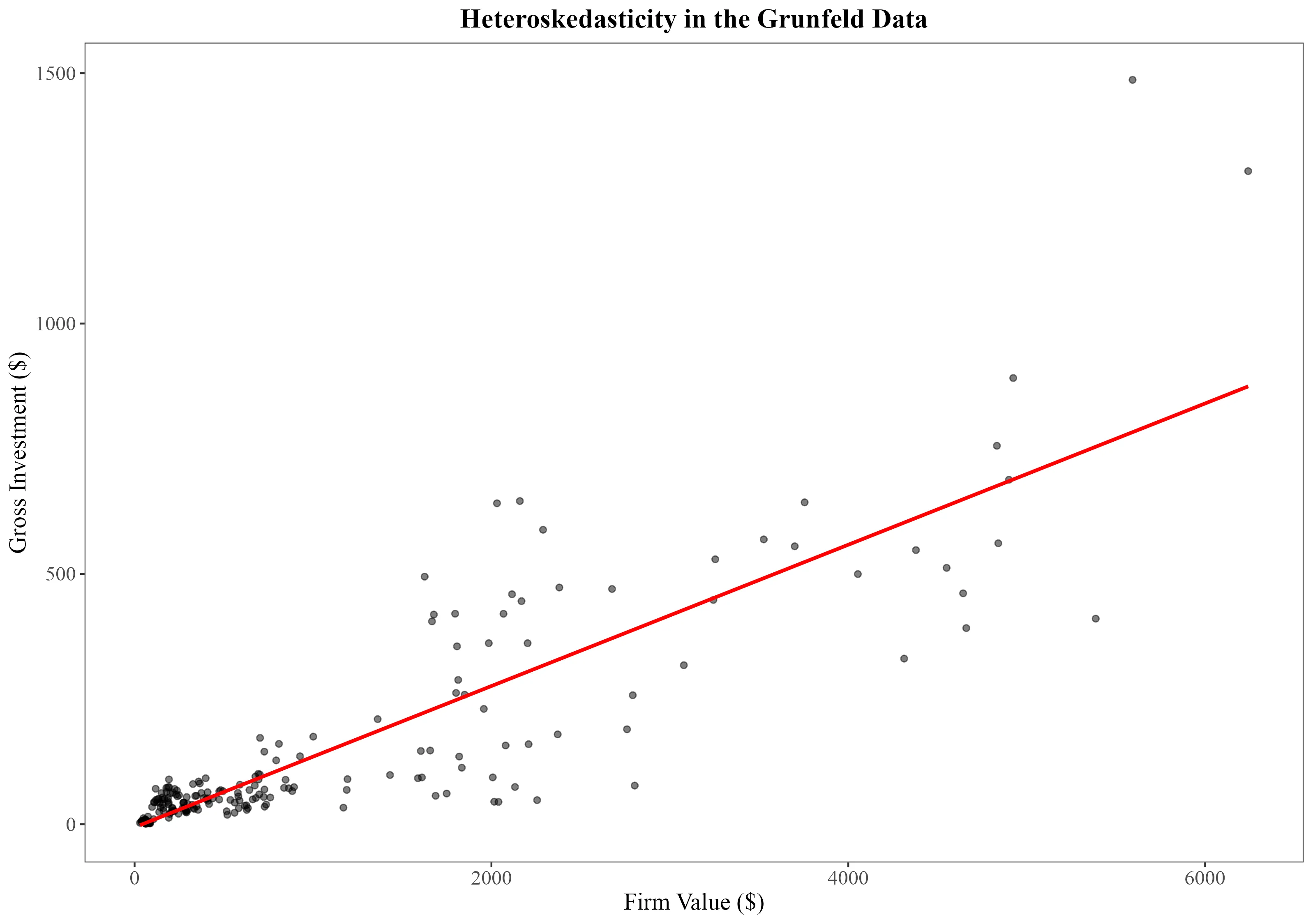
The first step to identify, whether heteroskedasticity is present in your data, is to visually inspect your data points around a regression line. This allows you to spot patterns of variance that might not be constant, such as fan-shaped or nonlinear distributions. Such patterns suggest that the variability of the residuals changes with the level of the independent variable.
By plotting the relationship between firm size (value) and gross investment (invest), we can examine whether the hypothesis that larger firms have more variance in their investment compared to smaller firms holds.
library(ggplot2)

# Scatter plot with a regression line
ggplot(Grunfeld, aes(x = value, y = invest)) +
  geom_point(alpha = 0.5) +
  geom_smooth(method = "lm", se = FALSE, color = "red") +
  labs(title = "Heteroskedasticity in the Grunfeld Data",
       x = "Firm Value ($)",
       y = "Gross Investment ($)") +
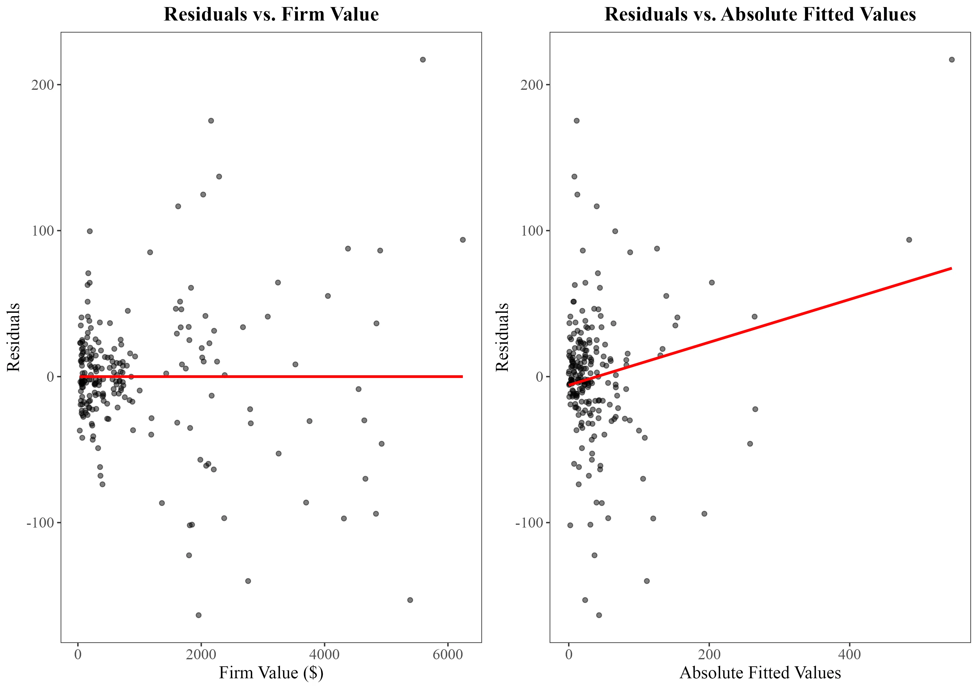
A more direct approach to investigate the presence of heteroskedasticity involves plotting your regression's residuals. This can be done against either the independent variables suspected of causing heteroskedasticity or against the regression's fitted values.
Here, both options, the residuals against the dependent variable and the residuals against the fitted value, are shown for the Grunfeld regression model:
# Create a new dataframe for visualization
dataframe <- data.frame(
  Value = Grunfeld$value,                 # Independent variable
  Residuals = residuals(grunfeld_model),  # Extract residuals from the regression model
  Fitted = fitted(grunfeld_model)         # Extract fitted values from the regression model
)

# Plot of residuals against the independent variable
ggplot(dataframe, aes(x = Value, y = Residuals)) +
  geom_point() +
  labs(title = "Plot of Residuals vs. Independent Variable")

# Plot of residuals against fitted values
ggplot(dataframe, aes(x = Fitted, y = Residuals)) +
  geom_point() +
  labs(title = "Plot of Residuals vs. Fitted Values")
Tests For Heteroskedasticity
Common tests for detecting heteroskedasticity are the Breusch-Pagan (BP) and the White test. A third test that will be discussed is the Goldfeld-Quandt test, which is suitable for regressions where indicator (categorical) variables are suspected to cause heteroskedasticity.
 Tip
TipBefore conducting these tests, it's advisable to check for and address any serial correlation in the data. The presence of serial correlation can invalidate the tests for heteroskedasticity. How to check for serial correlation is discussed in this article.
Breusch-Pagan (BP) Test
The Breusch-Pagan (BP) test is a statistical way used to test the null hypothesis that errors in a regression model are homoskedastic. Rejecting the null hypothesis indicates the presence of heteroskedasticity.
Steps to Perform the Breusch-Pagan Test:
- Run the Original Regression Model: Fit the original regression and compute the residuals.
$Y_i = \beta_0 + \beta_1 X_i + ... + \beta_k X_k + \epsilon_i$
- Optional: Perform the Auxiliary Regression
- Square the residuals from Step 1 and regress these squared residuals on the original independent variables.
- The benefit of taking this step is the identification of the variable(s) causing heteroskedasticity.
$\hat{u}{^2} = c_0 +c_1 x_1 +... + c_k x_k + \epsilon_i$
The dependent variable here, $\hat{u}^2$, represents the squared residuals.
- Calculate the BP Statistic 1. Reject the null hypothesis if the p-value is less than 0.05.
Implementation in R
library(lmtest)

# Step 1: Run the original regression model
grunfeld_model <- plm(invest ~ value + capital, data = Grunfeld, index = c("firm", "year"), model = "within", effect = "twoways")

# Optional: Step 2: Perform the second regression
uhat <- resid(grunfeld_model)  # Extract residuals
uhatsq <- uhat^2  # Square residuals
uhatsq_reg <- plm(uhatsq ~ value + capital, data = Grunfeld, index = c("firm", "year"), model = "within", effect = "twoways")
summary(uhatsq_reg)$coefficients

# Step 3: Execute the Breusch-Pagan (BP) test
bptest(grunfeld_model)
Variable Specific Coefficients
| Estimate | Std. Error | t-value | Pr(>t) | |
|---|---|---|---|---|
| value | 2.897796 | 1.064235 | 2.722892 | 0.007080514 |
| capital | 7.780105 | 1.732049 | 4.491850 | 0.00001230574 |
Breusch-Pagan Test
| statistic | p.value | parameter | method |
|---|---|---|---|
| 65.22801 | 0 | 2 | studentized Breusch-Pagan test |
ExampleThe significant BP test statistic rejects the null hypothesis of homoskedasticity, implying the presence of heteroskedasticity. Zoomed in, both value and capital show significant coefficients, suggesting that these variables significantly influence the variance of the residuals.
TipWhen your argumentation suggests that heteroskedasticity is only linked to certain independent variables within a model, it is a better practice to apply the Breusch-Pagan test to these variables, rather than regressing the squared residuals on all predictors.
The White Test
The White test is similar to the Breusch-Pagan test but is able to test for non-linear forms of heteroskedasticity.
Characteristics are:
- No Pre-defined Variance Form: Unlike the Breusch-Pagan test, which requires a predefined functional form for the variance.
- Variable Handling: Uses both the squares and cross-products of explanatory variables in the auxiliary regression.
- Able to detect more complex forms of heteroskedasticity, for example, that may not be linearly related to the explanatory variables.
- Robustness vs. Sample Size: While the White test is able to identify several heteroskedastic functional forms, it suffers from reduced power in smaller sample sizes.
- This is due to the inclusion of the squares and cross-products of explanatory variables in the auxiliary regression, which increases the degrees of freedom used. In small samples, this can make the test less effective, as the limited data points are distributed across more estimated parameters.
Steps to Perform the White Test:
- Run the Original Regression Model Fit the original regression and compute the residuals:
$Y_i = \beta_0 + \beta_1 X_i + ... + \beta_k X_k + \epsilon_i$
- Optional: Perform the Auxiliary Regression Regress the squared residuals on all explanatory variables, their squares, and cross products.
$\hat{u}{^2} = c_0 +c_1 x_1 + c_2 x_2 +c_3 x_1^2 + c_4 x_2^2 + c_5 x_1 * x_2 + \epsilon_i$
- Calculate the White Statistic
Implementation in R
library(whitestrap) # Used for the white_test() function

# Step 1: Run the original regression model
grunfeld_model <- plm(invest ~ value + capital, data = Grunfeld, index = c("firm", "year"), model = "within", effect = "twoways")

# Optional: Step 2: Perform the second regression
uhat <- resid(grunfeld_model)  # Extract residuals
uhatsq <- uhat^2  # Square residuals
uhatsq_reg <- plm(uhatsq ~ value + capital +I(value^2) + I(capital^2) + I(value * capital), data = Grunfeld, index = c("firm", "year"), model = "within", effect = "twoways")
summary(uhatsq_reg)$coefficients

# Step 3: Execute the White test
white_test(reg)
Variable Specific Coefficients
| Variable | Estimate | Std. Error | t-value | Pr(>t) |
|---|---|---|---|---|
| $value$ | -0.5964300241 | 2.5570433783 | -0.2332499 | 0.8158253 |
| $capital$ | -5.2861026172 | 4.5169926545 | -1.1702704 | 0.2433975 |
| $I(value{^2})$ | 0.0004999913 | 0.0003524792 | 1.4184988 | 0.1577276 |
| $I(capital{^2})$ | 0.0168003951 | 0.0031235152 | 5.3786821 | 0.0000002247362 |
| $I(value * capital)$ | -0.0039096384 | 0.0012232103 | -3.1962112 | 0.001637626 |
White Test
| Description | Value |
|---|---|
| Null hypothesis | Homoskedasticity of the residuals |
| Alternative hypothesis | Heteroskedasticity of the residuals |
| Test Statistic | 55.31 |
| P-value | < 0.0001 |
Goldfeld-Quandt Test
The Goldfeld-Quandt test is suited for models that include categorical variables or where data segmentation based on a specific criterion is used. It uses a split-sample approach to test for differences in variance across these segments.
Test Setup:
- Data Segmentation: Data are divided into two groups based on a predetermined criterion.
- In our example, we split firms into 'small' and 'large' based on the 85th percentile of firm size or use a categorical factor such as industry type.
- Hypotheses Formulation: $H_0: \sigma^2_1 = \sigma^2_0, \quad H_A: \sigma^2_1 \neq \sigma^2_0$
Implementation in R
The gqtest() function from the lmtest package in R is designed to perform the Goldfeld-Quandt test. It requires several parameters:
- formula: The regression model to test.
- point: Specifies the percentage of observations for the split.
- alternative: Can be "greater", "two.sided", or "less".
- order.by: Determines how the data should be ordered for the test.
- data: The dataset being used.
# Run the Goldfeld-Quandt test
GQ_test <- gqtest(formula = grunfeld_model,
                  point=0.85,
                  alternative="greater",
                  order.by= grunfeld$value)
Goldfeld-Quandt Test
| df1 | df2 | Statistic | p.value | Method | Alternative |
|---|---|---|---|---|---|
| 30 | 184 | 6.649377 | 0 | Goldfeld-Quandt test | variance increases from segment 1 to 2 |
ExampleThe outcome of the Goldfeld-Quandt test conducted on the 'Grunfeld' data indicates significant heteroskedasticity. This suggests that the variance in errors increases significantly from the smaller firms to the larger firms, supporting the presence of heteroskedasticity across firm sizes.
 Warning
So far, we have interpreted a rejection of the null hypothesis of homoskedasticity by the tests as evidence for heteroskedasticity. However, this may be due to an incorrect form of the model. For example, omitting quadratic terms or using a level model when a log model is appropriate could lead to a falsely significant test for heteroskedasticity.
Corrections for Heteroskedasticity
The presence of heteroskedasticity in a regression model makes the standard errors estimated incorrect and therefore needs to be corrected. Common practice is to use heteroskedasticity-consistent standard error (HCSE) estimators, often referred to as robust standard errors.
Robust standard errors are often considered a safe and preferred choice because they adjust for heteroskedasticity if it is present. If your data turns out to be homoskedastic, the robust standard errors will be very similar to those estimated by conventional OLS.
Robust Standard Errors in R
The vcovHC function from the sandwich package estimates heteroskedasticity-consistent covariance matrices of coefficient estimates, known as White's correction. his method adjusts the covariance matrix of the estimated coefficients to account for the impact of heteroskedasticity, thereby providing more accurate standard errors.
The vcovHC function in R provides different versions of heteroskedasticity-consistent standard errors:
- HC0 is the basic form without small sample adjustments.
- HC1 adds a degree of freedom adjustment.
- This adjustment makes HC1 a more reliable choice in practice, particularly in small-sized samples.
- HC2: Adjusts the errors based on the leverage values (how much influence each data point has on the regression).
- Suited for regressions with influential data points.
- HC3: Squares the adjustment factor used by HC2, making it more robustness against influential points.
- Recommended when sample sizes are small or the data contains outliers.
# Original Regression Model
grunfeld_model <- plm(invest ~ value + capital, data = Grunfeld, index = c("firm", "year"), model = "within", effect = "twoways")
summary(grunfeld_model)

# Correct to heteroskedasticity-consistent covariance matrix using White's method
robust_variance <- vcovHC(grunfeld_model, type = "HC1")

# Use the robust variance matrix to compute corrected standard errors, t-values, and p-values
corrected_reg <- coeftest(grunfeld_model, vcov = robust_variance)
Non-Corrected Model
| Variable | Estimate | Std. Error | t-value | Pr(>t) |
|---|---|---|---|---|
| value | 0.116681 | 0.012933 | 9.0219 | < 2.2e-16 *** |
| capital | 0.351436 | 0.021049 | 16.6964 | < 2.2e-16 *** |
Heteroskedasticity Corrected Model
| Variable | Estimate | Std. Error | t value | Pr(>t) |
|---|---|---|---|---|
| value | 0.116681 | 0.010451 | 11.1643 | < 2.2e-16 *** |
| capital | 0.351436 | 0.043610 | 8.0586 | 8.712e-14 *** |
Dealing with Serial Correlation and Heteroskedasticity
If your data consists of both serial correlation and heteroskedasticity, it;s necessary to use robust standard errors that correct for both. Again the vcovHC function allows for various types of robust covariance estimators. For models with time series data, consider using Arellano robust standard errors, which provide consistent standard errors in the presence of both heteroskedasticity and serial correlated errors:
grunfeld_model <- plm(invest ~ value + capital, data = Grunfeld, index = c("firm", "year"), model = "within", effect = "twoways")

# Abstract Arellano Covariance Matrix
arellano_robust_covariance <- vcovHC(grunfeld_model, method = "arellano", type = "HC3")

# Compute Arellano robust standard errors
summary_arellano <- summary(grunfeld_model, vcov = arellano_robust_covariance)
print(summary_arellano)
| Estimate | Std. Error | t-value | Pr(>t) | |
|---|---|---|---|---|
| value | 0.116681 | 0.012725 | 9.1698 | < 2.2e-16 *** |
| capital | 0.351436 | 0.059327 | 5.9237 | 1.473e-08 *** |
 Summary
This article explains how to detect and correct for heteroskedasticity in regressions using R. Explained using a practical example of the Grunfeld dataset, the following procedure is explained:
- Start, with a visual inspection of the residuals using ggplot2::ggplot() to identify variance patterns.
- Thereafter, use statistical tests such as Breusch-Pagan (lmtest::bptest()) and White test (whitestrap::white_test()).
- At last, if the tests indicate heteroskedasticity, corrections need to be applied, using robust standard errors through sandwich::vcovHC() or a new functional form of the model.