Overview
deltaMethod is a R function that approximates the standard error of a transformation $g(X)$ of a random variable $X = (x_{1}, x_{2},..)$, given estimates of the mean and the covariance matrix of $X$. The approximation is given by the formula:
$Cov(g(X)) = g'(\mu)Cov(X)[g'(\mu)]^T$, where $\mu$ is an estimate of the mean of $X$.
Having the regression coefficients might not be enough if we want to interpret some combined effects between them. Merely summing the coefficients does not ensure that the resulting effect is significant and it also does not offer any information on the resulting standard error.
To obtain the combined effects of coefficients we can use the deltaMethod function of the R car package. To illustrate how to implement it we use two example datasets: the "Boston Housing" dataset example available in the MASS package of R and the "hernandez.nitrogen" example, a dataset of an agricultural trial of corn with nitrogen fertilizer available in the agridat package.
Implementation
Example 1
Let's first load the Boston dataset and required packages.
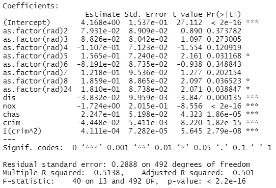
Next, we perform a non-linear regression analysis. We regress the natural logarithm of the medv variable, which is the median value of owner-occupied homes in $1000s, on :
rad: the index of accessibility to radial highways, included as factor variabledis: the weighted mean of distances to five Boston employment centresnox: the nitrogen oxide concentrationchas: the Charles River dummy variablecrim: per capita crime rate
#linear model
mod <- lm(log(medv) ~ as.factor(rad) + dis + nox + chas + crim + I(crim^2), data = Boston)

summary(mod)
Output:

Now let's calculate the combined effect of the first order crime rate per capita (crim) with the second order crim. The deltaMethod function takes as first argument the regression object, followed by the names of the coefficients between quotes:
Output:

We see that the combined effect of the two coefficients is -0.044, with a standard error of 0.005 and p-value smaller than .000, denoting that the resulting coefficient is significant at a 0.1% level.
Alternatively, we can calculate the effect of the Charles River dummy (chas) multiplied with the previous combination of first and second order crime rate per capita.
Output:

The output shows that the combined coefficient is -0.009, with a standard error of 0.003 and a 95% confidence interval between -0.016 and -0.003.
Example 2
For the second dataset, we first load the necessary libraries and the data.
This is a simple profit maximization problem: given the quantity of nitrogen and corn resulted, as well as input and sales prices, we aim to maximize the profit.
We first create an income variable by subtracting the costs of fertilization (nitro*input_price) from the revenue resulted from selling the corn (yield*sale_price):
income = yield*sale_price - nitro*input_price
sale_price <- 118.1
input_price <- 0.665

df <- df %>% mutate(income = yield*sale_price - nitro*input_price)
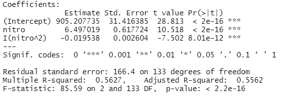
Next we run a quadratic regression between income as a dependent variable, and the nitrogen use as an independent variable.
Output:

We can now calculate the optimal nitrogen quantity given the prices and the resulted coefficients. We use the formula: $-nitro/(2*nitro^2)$.
deltaMethod(mod1, "-nitro /(2*`I(nitro^2)`)", rhs=1)

#equivalently we can also use the beta parameters
deltaMethod(mod1, "-b1/(2*b2)", parameterNames = paste("b", 0:2, sep = ""))
Output:

The optimum nitrogen quantity is 166, as shown by the significant estimate of the deltaMethod.


