Overview
The notion of a loss function is foundational for the training machine learning models.
It provides a quantitative measure of how well or poorly a model is performing.
Different kinds of machine learning tasks (classification or regression) and datasets may require specific loss functions to achieve optimal results.
Knowledge of the loss function is essential to minimize errors and enhance predictive accuracy.
In this article, we'll discuss the common cost functions used in both regression and classification problems. This knowledge will help you to select the most suitable cost function for your machine learning tasks.
The Loss Function vs the Cost Function!
These two terms are occasionally used interchangeably, but they are refer to different things. The loss function is the variance between the actual and predicted values for an individual entry in the dataset. The cost function is the average of the loss function across the entire dataset. The cost function is use in optimizing the best function for the training data.
Cost function in regression problems
Imagine fitting a simple line (Equation 1) to a dataset with a numeric target using two parameters, $\theta_0$ and $\theta_1$. The aim is to pick the right values for $\theta_0$ and $\theta_1$ so that the gap between the predicted value $h_\theta(x)$ and the actual value $y$ is minimum. This task needs to solve a minimization problem, where you minimize the cost function. You've got various choices for cost functions, that you'll be familiar with, in following sections.
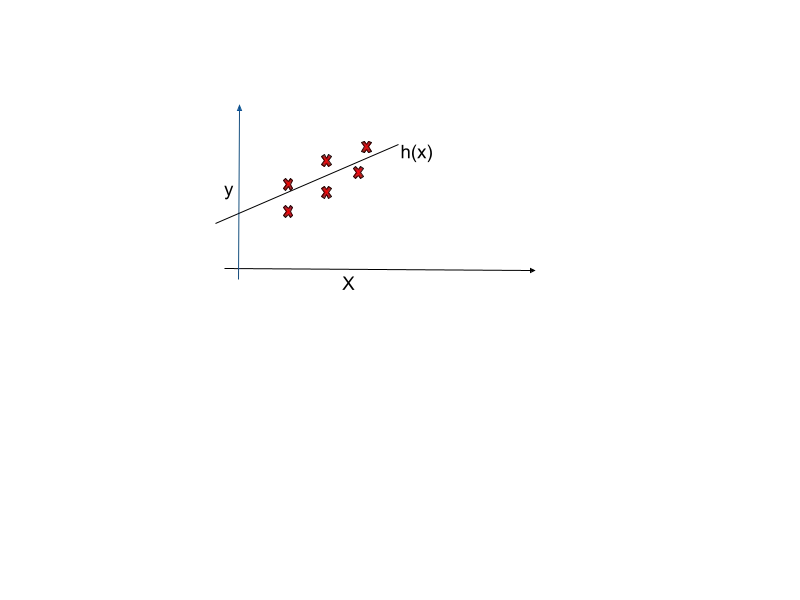
$h_\theta(x)$ is going to be objective function for linear regression.
Mean Squared Error (MSE)
One method involves minimizing the squared difference between $y$ and $h(x)$, then computing their average. In fact, this approach utilizes Mean Squared Error (MSE) as the cost function (Equation 2).
This cost function is widely used for optimizing the majority of regression problems. For a more intuitive understanding, let's consider the following example.
 Example
for simplicity, let's assume $\theta_0=0$, implying that the equation line passes through the origin $(0,0)$. Our goal is to fit the equation $h(x)=\theta_1*x$ to the sample data showed by red crosses in the following plots. We examine different values for $\theta_1$ such as $1, 0.5, -0.5$ to observe their efffect on the cost function $J(\theta_1)$. while $h_\theta(x)$ is a function of $x$, the cost function is dependent on $\theta_1$. The plots below illustrate how changes in $\theta_1$ values affect the cost function. Note that we need to find th optimal $\theta_1$ that minimize cost function.
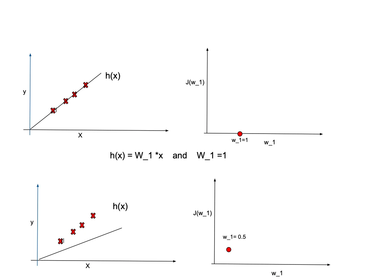
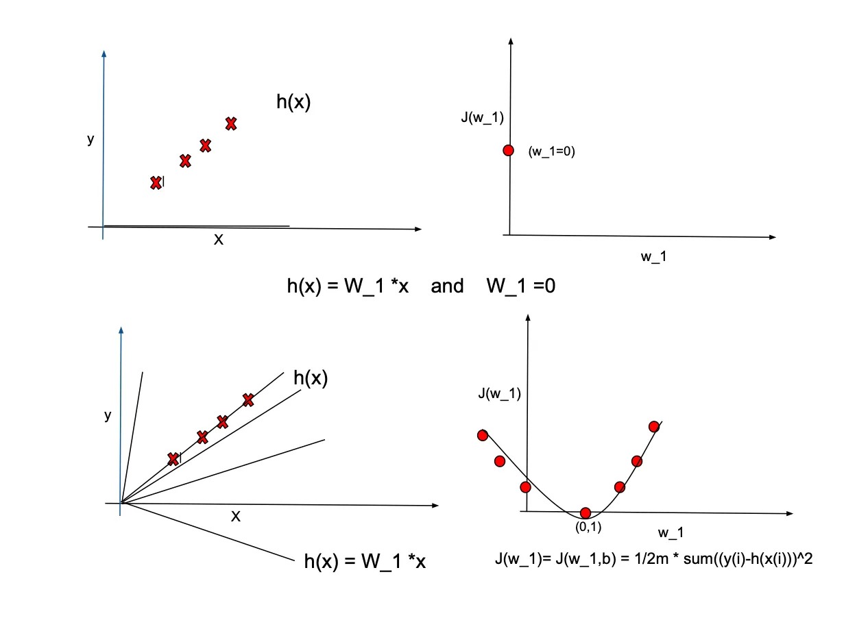
In real-world scenarios, it's common to have more than one predictors. Therefore, the cost function dependents on multiple variables. In the case of a two-dimensional problem, the cost function takes on a form similar to the following:
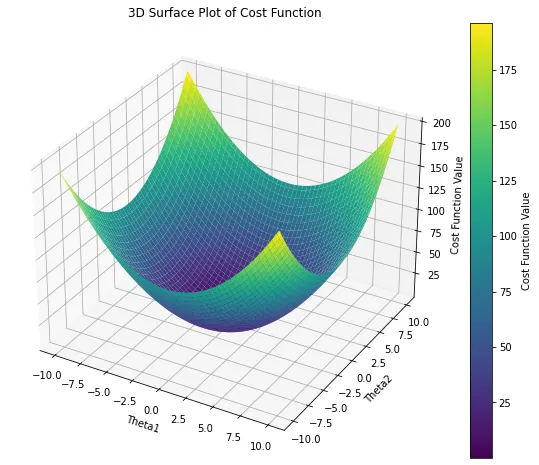
The contour plot below illustrates the two-dimensional cost function, representing the mapping of the previous plot onto a 2D surface. Each contour on this plot corresponds to the same cost value for different $\theta$ values. In machine learning, the goal is to navigate towards the smallest contour on this plot, indicating the minimum cost value. Essentially, when $\theta_1$ and $\theta_0$ are set in a way that the line aligns with the data trend, the cost value converges towards the center (minimum value). Conversely, when the objective function is not aligned with the data trend, the cost value is situated farther from the center on the contour levels. This alignment process is crucial in achieving optimal parameter values for effective model fitting.
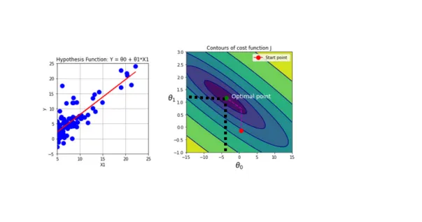 Contour map on cost function for two dimentional problem.
 Tip
Tip- MSE is also referred to as L2 loss.
- MSE is notably sensitive to outliers. In the presence of outliers within the dataset, the error tends to increase exponentially.
Ridge regression and lasso
There are two options available for mitigating overfitting in MSE: - Applying L2 regularization to the MSE equation. - Applying L1 regularization to the MSE equation.
When the L2 regularization term is added to the MSE, the resulting model is referred to as Ridge regression. In Ridge regression, the model faces a penalty if the coefficients become large,the regularization term acts to diminish the impact of coefficients, mitigating the risk of overfitting. The $\lambda$ term control the degree of regularization, with an increase in $\lambda$ intensifying regularization; typically, the default value is set to 1. In bellow formula $\lambda \sum_{j=1}^{p} \theta_j^2$ is the regularization term.
 Tip
TipAs the regularization strength increases, the coefficients' ($\theta$) decrease, yet they never reach zero.
By adding L1 regularization penalty term to the MSE, the equation is called lasso, short for Least Absolute Shrinkage and Selection Operator. Similar to the previous regurarization method, parameter $\lambda$ control the strength of regularization. But in this method many weights being precisely set to zero. Note that L1 regularization favors sparse models by encouraging coefficients to be exactly zero, facilitating automatic feature selection where some features are entirely ignored.
Mean Absolute Error(MAE)
This loss function also known as L1 loss. It gives the average of absolute errors of all data samples. In contrast to MSE that get the average of squared error, it takes the average of the absolute error. This characteristic makes it robust to the outliers. Therefore it is more suitable if your datasets contains outliers or noises.
 Tip
TipAlthough MAE is less sentative to outliers compared to the MSE, some times MSE is preffered since MAE is not diffrentiable.
Smooth Mean Absolute Error or Huber Loss
This cost function is the mixture of both previous cost functions. Hence, it is differentiable when the error is small by using the MSE part, and it uses MAE when the error is large. Therefore is less sensitive to the outliers and noise and differentiable close to the minima. There is a hyperparameter to tune it when use MSE or MAE.
Cost function in classification
Cost functions used in classification differ from those in regression models, primarily due to the nature of the target variable. In regression models, the target variable is continuous, whereas in classification problems, it is discrete. The most common cost function in classification is the cross-entropy loss, which comes in two variations: Binary Cross-Entropy for binary classification and Categorical Cross-Entropy for multiclass classification. Another commonly used cost function in classification is Hinge loss.
Cost Function for Binary Classification Tasks
In machine learning problems where the target variable has two classes, Binary Cross-Entropy is used. This loss function is alternatively referred to as log loss, logistic loss, and maximum likelihood. Additionally, L1/L2 regularization terms can be incorporated into this loss function.
Cost Function for Multiclassification models
In a classification problem with multiple classes as the target variable, it is necessary to use categorical cross-entropy as the loss function.
Hing loss
Another alternative is hinge loss, also referred to as Multi-class SVM Loss. This particular cost function is designed to maximize the marginal distance and is commonly used for optimizing Support Vector Machine (SVM) models.
The Hing loss equals zero when $x_i$ is positioned correctly with respect to the margin(it means when the prediction is correct). However, for data located on the incorrect side of the margin, the function's value is directly proportional to the distance from the margin.
By adding a regularization term to the equation, the parameter $\lambda > 0$ plays a crucial role in achieving a balance between enlarging the margin size and ensuring that $\max(0, 1 - y_i \cdot \hat{y}_i)$ is satisfied, guaranteeing that $x_i$ lies on the correct side of the margin.
 Example
Consider optimizing a logistic regression problem involving two classes, denoted as 0 and 1. In this context, the objective function is represented by the sigmoid function, which is outlined as follows:
and suitable cost function is Binary Cross-Entropy.
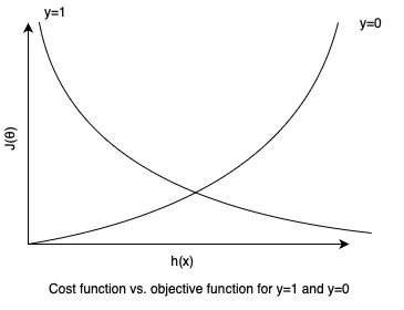
The next figure visualizes the cost function across various combinations of the predicted values($h_\theta(x)$) and actual labels when $y$ is either $0$ or $1$. This visualization provides insights into how the cost varies with different scenarios. For instance, when predicted value is $0$ while the actual value is $1$, the cost function goes towards infinity.
 Summary
- Definition of Cost and Loss function
- Cost functions aplicabple in regression problems - Mean Squared Error: Measures the average squared difference between predicted and actual values. - Ridge regresssion: Introduces regularization by penalizing large coefficients to prevent overfitting. - Lasso Regression: Another regularization technique penalizing the absolute size of coefficients. - Mean Absolute Error : Computes the average absolute difference between predicted and actual values. - Smooth Mean Absolute Error: An improved version of MAE with a smooth transition for small errors.
-
Cost functions applicable in classification problems - Binary Cross-Entropy: Used in binary classification tasks to quantify the difference between predicted and actual class probabilities. - Categorical Cross-Entropy: Suitable for multi-class classification, calculates the difference between predicted and actual class probabilities. - Hing Loss: Commonly used in support vector machines (SVMs) for binary classification, penalizing misclassified samples.
-
provided examples to enhance understanding of the concepts.


