Overview
In this article, our focus is on understanding and tackling overfitting issues that may emerge during the training of Decision Trees. We will delve into various techniques that can be employed to mitigate overfitting and enhance the model's generalization ability, equipping you with the tools to address this challenge effectively.
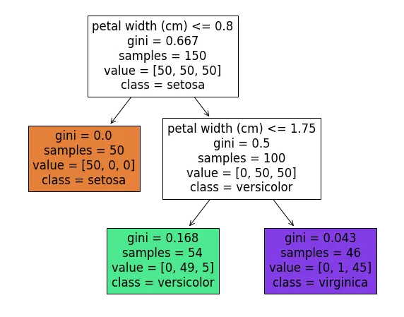
Think of the Decision tree as a map explaining to us how the model makes predictions. Looking at the following image, in depth1, left node, 50 samples with a petal width less than 0.8 cm are all setosa, showing petal width is excellent for identifying setosa. In other leaf nodes (depth2), petal width is used again; however, the Gini value is not zero this time, and some flower types are mixed. If we keep dividing, we might make purer groups, but there's a risk of overfitting. Overfitting is like trying too hard to fit everything perfectly, making the model less useful for new data that the algorithm has yet to see. In decision trees, overfitting occurs when leaf nodes have high purity, indicated by Gini values close to zero or zero in classification problems, and very low MSE in regression problems during training.

Overfitting
The decision tree algorithm is prone to overfitting because it has unlimited freedom. This means that the splitting of the tree continues until the classes are distinguished with zero impurity. To prevent overfitting, we can limit this freedom through hyperparameter tuning.
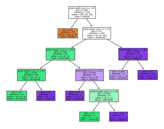
The code block trains a decision trees classifier with no restrictions. The resulting tree will have all leaf nodes with Gini impurity equal to 0, indicating a perfect fit to the data. However, this may lead to overfitting and poor performance on new data. It's worth noting that some leaf nodes may only have one or two samples, making the tree less generalizable.
 Tip
TipGini impurity is used to identify the ideal attribute to split on. Gini impurity measures how often a randomly chosen attribute is misclassified. When evaluating using Gini impurity, a lower value is more ideal. Gini impurity is zero when a node is included only one class.
from sklearn.datasets import load_iris
from sklearn.tree import DecisionTreeClassifier

# Load data from Sklearn datasets
iris = load_iris()
X = iris.data[:, 2:]
y=  iris.target

# train a DT classifier
DT_clf = DecisionTreeClassifier()
DT_clf.fit(X,y)

Take note of the following text:
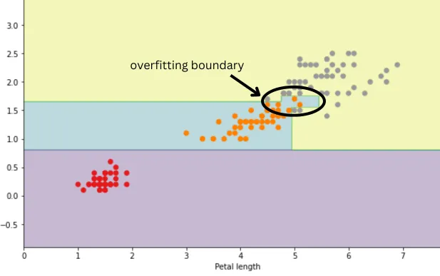
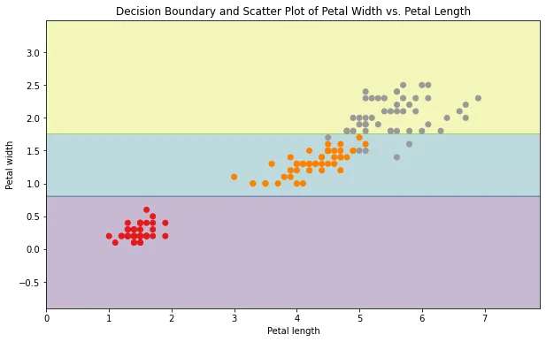
When you compare the decision boundaries in the two images below, you'll notice the impact of overfitting. In the unconstrained model, the decision boundary is positioned to perfectly separate the classes, indicating overfitting. To tackle this issue, smoother boundaries are needed, allowing for imperfect separation of the training data and not requiring every single sample to be correctly classified.


Mitigating Overfitting in Decision Trees Classifier
A standard method for addressing overfitting in decision trees is pruning. Pruning cuts portions of the tree, preventing it from expanding to its maximum depth. For example, consider separating the flower classes based on petal width and petal length using a decision tree algorithm.
In Figure 1, pruning restricts the tree's growth, preventing it from reaching its maximum possible depth, leaf, and nodes. So, the splitting of the classes continues until the restriction on the tree growth, like the maximum depth of growth, is reached.
Conversely, in Figure 2, the splitting of the flower classes continues until all flowers are assigned to the correct class. This is because there is no restriction on the splitting and tree growth, leading to an unrestricted expansion of the tree.
There are generally two types of pruning: pre-pruning and post-pruning. Pre-pruning involves adjusting hyperparameters in the model. In this approach, pruning occurs during the training phase by setting conditions for the training to stop. This method allows you to control the model's complexity. The second method is post-pruning, which we will explore further.
Pre-Pruning and Hyperparameter Tuning
The hyperparameters that can be adjusted in a Decision Tree classifier to combat overfitting include:
-
Maximum depth of Decision Tree: Reducing depth of the tree decreases the likelihood of overfitting. The
max_depthparameter is a common way to control the decision tree. Increasing this parameter will lead to a model that fits the training data more. Feel free to experiment with different values and compare the results. -
Minimum number of samples per node: Setting a minimum number of samples per node ensures that the model avoids splitting a node if the number of samples falls below a certain threshold. In
Sklearn,the default value for this parameter is None. -
Minimum number of samples per leaf: Remember the example in Figure-2 in which some leaf nodes have a few samples. To enhance the model, you can avoid leaf nodes with very few samples by assigning a threshold to this parameter. It helps decrease the chance of overfitting.
-
Maximum number of leaf nodes: By setting this parameter, the tree prevents the creation of an excessive number of leaf nodes, halting when it reaches the specified threshold. Reducing the value of this parameter helps the model become more generalized.
-
Maximum number of features for splitting a node: This parameter refers to the maximum number of features the algorithm considers when looking for the best split at each node. The model becomes too complex when the number of features is high and the number of samples is low. In the context of decision trees, allowing the algorithm to consider too many features for splitting can lead to overly complex trees that capture noise in the data.
All the abovementioned strategies are called pre-pruning techniques, in which the trees don’t grow more when they reach a pre-defined threshold. These methods are simple, easy to implement, and computationally efficient.
By constraining the model, you are making a conscious trade-off: the training accuracy decreases, but the model becomes simpler and can fit better on the test data. This awareness of the trade-off and the need to tune the parameters to balance these two aspects is crucial in achieving a model with acceptable accuracy and simplicity.
By setting the maximum depth of a decision tree, you can effectively manage the model and eliminate the requirement for additional thresholds. When we restrict the maximum depth of the decision tree, other parameters, like the Maximum number of leaf nodes, also go under limitation.
Here are some guidelines that can help you to set the maximum depth effectively:
1- Start with a low maximum depth, such as 3 to 5 levels, to keep the model simple and prevent it from capturing noise in the training data. Then, gradually increase the depth to observe how the model's performance changes on the validation set.
2- Visualizing the decision tree can help identify complex branches that might contribute to overfitting. Simplify the tree by reducing the depth or pruning branches that do not significantly improve performance.
3—Shallower trees are generally preferred for smaller datasets to avoid overfitting. Deeper trees can be explored for larger datasets with more variability, but still with caution.
Post-pruning
This approach is also known as backward pruning or cost-complexity pruning. This technique involves growing the tree to its maximum size and then removing or collapsing nodes that contribute little to the overall predictive accuracy of the tree.
 Tip
TipBy applying pruning, the training accuracy may decrease but significantly affect the overfitting.
Cost Complexity Proning
Let's consider a classification problem. You can use wine dataset from the Sklearn library to follow the steps.
# import libraries
from sklearn.datasets import load_wine
from sklearn.model_selection import train_test_split
from sklearn.tree import DecisionTreeClassifier
from sklearn.metrics import accuracy_score

# load data
wine = load_wine()
X = wine.data
y = wine.target

# Split the dataset into training and testing sets
X_train, X_test, y_train, y_test = train_test_split(X, y, test_size=0.2, random_state=1)

# Decision Tree classifier
dt_clf = DecisionTreeClassifier()
dt_clf.fit(X_train, y_train)

# Make predictions on the train and test set
train_pred = dt_clf.predict(X_train)
test_pred = dt_clf.predict(X_test)

# Calculate accuracy on the train and test set
train_accuracy = accuracy_score(y_train, train_pred)
print("Accuracy for train set:", train_accuracy)

test_accuracy = accuracy_score(y_test, test_pred)
print("Accuracy for test set:", test_accuracy)
After running the above code, you get a training accuracy of 1 and a test accuracy of 0.88. This indicates an overfitted model. To address this, we'll introduce the Cost Complexity Pruning algorithm.
The Cost Complex Proning algorithm, also called Weakest Link Proning, determines how many branches of the tree to prune. The first step is to find each tree's error rate (the Gini value in classification and the Sum of Squared Residuals in regression). It starts with a full-size tree, calculates the error, and continues by calculating the subtrees' error each time by removing one node leaf. It will continue until only one node remains.
The error in the first tree, a full tree with the maximum possible leaf node and maximum possible depth is minimum and gets larger by pruning the tree. We aim to find a tree with balanced accuracy and simplicity. To do that, we calculate the Tree Score based on the total misclassification rate($R$), a Tree Complexity Penalty that is a function of the number of leaf nodes ($T$) and $\alpha$. $\alpha$ is a tuning parameter named Cost complexity Proning, and we find it using cross-validation. We repeat calculating $Tree Score$ for different $\alpha$. Note that different $\alpha$ gives a different tree as the best tree. We are looking for the tree with the minimum value of Tree Score.
 Tip
TipTree Complexity Penalty for trees with more leaf nodes is larger.
# finding alpha by cross-validation and using all samples
path = dt_clf.cost_complexity_pruning_path(X, y)
ccp_alphas, impurities = path.ccp_alphas, path.impurities

# training the classifier with different alphas and append the list of classifiers
clfs = []
ccp_alphas = ccp_alphas[:-1] # After removing the trivial tree with only one node
for ccp_alpha in ccp_alphas:
    clf = DecisionTreeClassifier(random_state=0, ccp_alpha=ccp_alpha)
    clf.fit(X_train, y_train)
    clfs.append(clf)
 Tip
TipDon't forget to use all samples, including train and test data in the step of finding alpha's
Now, you have a list of classifiers with different alpha and accuracy. The following code block to visualize the training and testing accuracies of different models versus alpha.
train_scores = [clf.score(X_train, y_train) for clf in clfs]
test_scores = [clf.score(X_test, y_test) for clf in clfs]

fig, ax = plt.subplots()
ax.set_xlabel("alpha")
ax.set_ylabel("accuracy")
ax.set_title("Accuracy vs alpha for training and testing sets")
ax.plot(ccp_alphas, train_scores, marker="o", label="train", drawstyle="steps-post")
ax.plot(ccp_alphas, test_scores, marker="o", label="test", drawstyle="steps-post")
ax.legend()
plt.show()
Now, it's time to find the optimum alpha and train your model using it.
# find alpha with less overfitting model
scores = list(zip(train_scores,test_scores))
min_index = min(range(len(scores)), key=lambda i: abs(scores[i][0] - scores[i][1]))
print("Index with minimum overfitting:", min_index)

optimum_alpha = ccp_alphas[min_index]
print("optimum alpha:",optimum_alpha)
Now, train the model with optimum alpha.
# train the model with optimum alpha
dt_clf_optimum = DecisionTreeClassifier(random_state=0, ccp_alpha=optimum_alpha)
dt_clf_optimum.fit(X_train, y_train)

# Make predictions
train_pred = dt_clf_optimum.predict(X_train)
test_pred = dt_clf_optimum.predict(X_test)

# Calculate accuracy on the train and test set
train_accuracy = accuracy_score(y_train, train_pred)
print("Accuracy for train set:", train_accuracy)

test_accuracy = accuracy_score(y_test, test_pred)
print("Accuracy for test set:", test_accuracy)
Thanks to the effectiveness of the Cost Complexity Pruning algorithm, you now have a less overfitted decision tree with training and testing acuracies of 0.88 and 0.86.
Let's compare the tree from the optimum classifier and the tree from the model with no limitations.
from sklearn.tree import plot_tree
import matplotlib.pyplot as plt

# Visualize the optimum trained decision tree
plt.figure(figsize=(10, 8))
plot_tree(dt_clf_optimum, filled=True, feature_names=wine.feature_names, class_names=wine.target_names,)
plt.show()

# Visualize the unrestricted trained decision tree
plt.figure(figsize=(15, 12))
plot_tree(dt_clf, filled=True, feature_names=wine.feature_names, class_names=wine.target_names,)
plt.show()
It's worth noting that cost Complexity Pruning is a more resource-intensive method compared to pre-pruning techniques. And, it is more useful in classification tasks compared to regression tasks.
 Summary
- Overfitting in Decision Trees
- How it appears in the tree diagram
- Why it happens
- Hyperparameter tuning to get a more generalized model
- Introducing different parameters in Decision trees algorithm
- Post-proning technique
- Cost Complexity Proning algorithm
- An example of implementing Cost Complexity Proning algorithm in a classification problem


