Overview

This article is a follow-up to Get Introduced to Machine Learning, which covered the basics of different machine learning types. In this article, we will dive deeper into one of the types of machine learning: Unsupervised Learning.

This in-depth introduction to unsupervised learning will cover its key concepts, algorithms and provide hands-on examples in R to illustrate how you can use these concepts in practice. Whether you are new to this topic, only have basic coding skills or just curious about unsupervised learning - this article will equip you with the tools to start your first unsupervised learning model.

The article covers several topics:

1. What is Unsupervised Learning?
2. Unsupervised Learning Algorithms
3. A Clustering Example
4. An Association Example
5. A Dimensionality Reduction Example

What is Unsupervised Learning?

This type of machine learning learns from data without human supervision. These models can detect previously unknown patterns in datasets without specified labels or outcomes. It uses self-learning algorithms to structure information based on similarities, differences, and patterns in data. Unsupervised learning approaches are often used to find structure in large datasets, and create a more compact representation of the data that is easier to understand.

Different approaches are clustering, association, and dimensionality reduction:

• Clustering
• Association
• Dimensionality Reduction

Clustering

Clustering organizes data by grouping similar data points together. Because members of the same group tend to have similar characteristics, clustering algorithms can group unlabeled data based on their similarities and differences. The goal is to have similar data points in the same cluster, and different data points in different clusters. Clustering algorithms are widely used in market research, customer segmentation, fraud detection, and image analysis. For example, on LinkedIn, clustering can be used to discover professional communities based on shared interests, job roles, or industry sectors, such as “technology innovators” or “digitial marketing professionals”.

Association

Association rule mining is used to uncover patterns and relationships in the data. It does so by finding rules that represent large parts of the data. It discovers correlations, connections, and co-occurences, and is often used to track purchases or make recommendations to customers. For example, Netflix uses association algorithms to discover that people who watch certain genres like science fiction often also enjoy fantasy series, and they can recommend new shows based on viewing habits.

Dimensionality Reduction

Dimensionality reduction techniques are used to reduce the number of input variables in a dataset. It removes irrelevant or random features while maintaining as much important information as possible. This can help increasing the efficiency of future analyses, reduce computational costs, and help with the visualization and interpretability of the data. In other words, it is a process of transforming high-dimensional data into a lower-dimensional dataset that still captures the essence of the original data. Dimensionality reduction algorithms are usually used as a pre-processing step in modeling, before the actual model training.

Unsupervised Learning Algorithms

Clustering

• K-Means Clustering

  • This algorithm segments data into groups based on similarity and common attributes. The dataset is divided into K clusters by minimizing the distance between each data point and the cluster centroid (central point within the cluster). An example is segmenting customers into distinct groups based on their purchasing behavior.

• Hierarchical Clustering

  • Hierarchical clustering does not require the number of clusters (K) to be specified in advance. It builds a hierarchy either by starting with all data points as one group and splitting them (divisive method), or by starting each data point as its own group and combining them (agglomerative method).

• Anomaly Detection

  • This method finds data points that differ significantly from the rest of the data. In fields like fraud detection, anomaly detection helps in spotting unusual transactions that could be fraud.

Association

• Apriori Algorithm

  • This association rule algorithm is great for discovering relationships between variables in large databases. It can find frequent itemsets in transactional data, such as identifying products that frequently get bought together.

• Eclat Algorithm

  • Eclat locates frequently occurring itemsets in transactional databases by performing a depth-first search. It speeds up the process and reduces computational costs by using a vertical data format that lists each item along with its transaction ID.

Dimensionality Reduction

• Principal Component Analysis (PCA)

  • PCA reduces the dimensionality of data by transforming the original variables into a new set of variables, which are linear combinations of the original variables. It simplifies data without losing its core information, and is useful in visualizing high-dimensional data.

• Linear Discriminant Analysis (LDA)

  • LDA separates multiple classes with multiple features by identifying a linear combination of features that separates two or more classes. It projects data with two or more dimensions into one dimension, so that it can be more easily classified. It is often used as a pre-processing step of classification algorithms like decision trees.

A Clustering Example: K-Means Clustering

In this example of clustering in unsupervised learning we will use the iris dataset. This dataset consists of measurements of iris flowers from three different species. Here is how you can apply K-means clustering to this dataset in R.

Loading and Preparing the Data

First, we load and prepare the data by removing labels since K-means is an unsupervised technique:

Determine the Number of Clusters

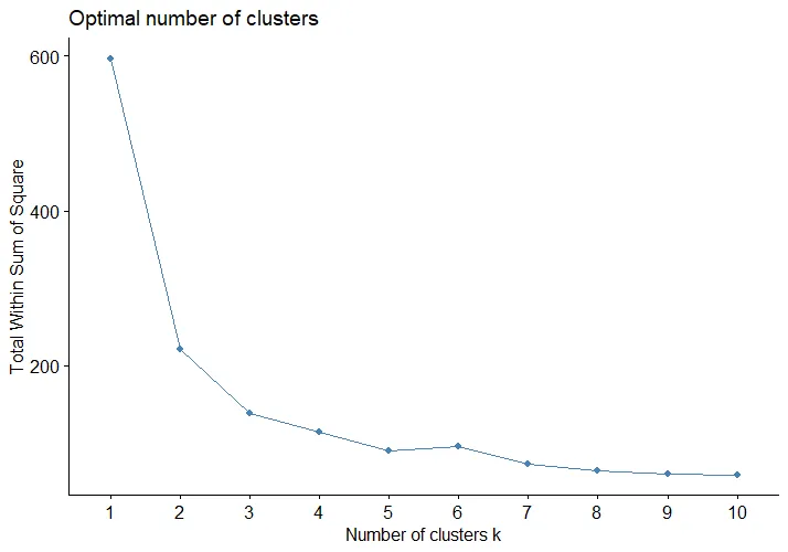
Next, we use the Elbow Method to determine the optimal number of clusters:

In the image, we can see that the elbow is at k=3.

Running K-Means Clustering

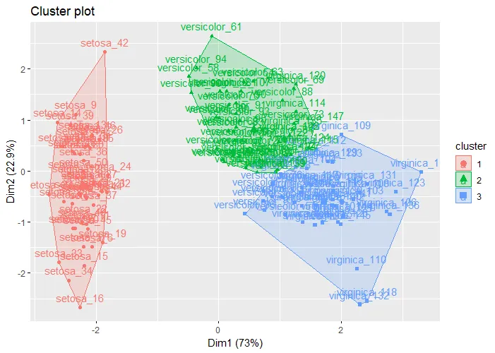
We can now proceed with the actual clustering. We choose our number of clusters (k=3) with centers = 3. Once we ran the algorithm, we need to check how well the model did by putting back the labels from the removed Species column. We can then visualize the clustering results:

The plot visually shows us how well the model did. The colours show to clusters that the algorithm made. The labels (in text) show the actual labels. We can see that most flowers are correctly labeled, but some are not:

Analyzing the Results

Finally, we compare the clusters with the original labels to see how well our clustering matched the actual species distribution:

Cluster	Setosa	Versicolor	Virginica
1	50	0	0
2	0	48	14
3	0	2	36

The results show that:

• Cluster 1 exclusively contains all 50 Setosa samples.
• Cluster 2 primarily contains Versicolor, with 48 out of 50, but also includes 14 Virginica.
• Cluster 3 mostly contains Virginica, with 36 out of 50, but includes 2 Versicolor.

An Association Example: Apriori Algorithm

In this example of association rule mining, we will use the Groceries dataset from the arules package in R. This dataset contains transactions from a grocery store, where each transaction lists the items purchased together by a customer.

Loading the Data

First, we load and inspect the data from the arules package. In this example, no preprocessing is needed, because the Groceries dataset is already in the right format for association rule mining:

Mining Frequent Itemsets

Using the Apriori algorithm, we identify the most commonly purchased itemsets. We need to specify the minimum support - we choose a support of 1% with supp = 0.01:

Here we see the top 5 bought items based on their support in the dataset. For example, whole milk is bought in a quarter of all transactions:

Rank	Item	Support	Transaction Count
1	Whole Milk	25.55%	2513
2	Other Vegetables	19.35%	1903
3	Rolls/Buns	18.39%	1809
4	Soda	17.44%	1715
5	Yogurt	13.95%	1372

Creating Association Rules

Next, we generate association rules from these frequent itemsets. We need to specify the minimum confidence - we choose a confidence of 50% with conf = 0.5:

Here are the top 5 rules with our chosen support and confidence levels:

#	Antecedent (LHS)	Consequent (RHS)	Support	Confidence	Coverage	Lift	Count
1	{Citrus Fruit, Root Vegetables}	{Other Vegetables}	1.037%	58.62%	1.769%	3.030	102
2	{Tropical Fruit, Root Vegetables}	{Other Vegetables}	1.230%	58.45%	2.105%	3.021	121
3	{Curd, Yogurt}	{Whole Milk}	1.007%	58.24%	1.729%	2.279	99
4	{Other Vegetables, Butter}	{Whole Milk}	1.149%	57.36%	2.003%	2.245	113
5	{Tropical Fruit, Root Vegetables}	{Whole Milk}	1.200%	57.00%	2.105%	2.231	118

• Antecedent (LHS): Items that customers often buy together. For example, in the first row, we see that “Citrus Fruit and Root Vegetables” are often bought together
• Consequent (RHS): An additional item that is frequently purchased with the itemset in the Antecedent column. For instance, when customers bought “Citrus Fruit and Root Vegetables”, they also often bought “Other Vegetables”.
• Support: How often the rule applies to the total number of transactions. For example, the first support of 1.037% means that in just over 1% of all transactions, customers bought citrus fruit, root vegetables, and other vegetables together.
• Confidence: How often the rule has been found to be true. For the first rule, 58.62% of the time when both citrus fruit and root vegetables were bought, other vegetables were also purchased. This shows how reliable the rule is.
• Coverage: The percentage of all transactions that include the Antecedent (the initial set of items). So, 1.769% of all transactions at the store included both citrus fruit and root vegetables.
• Lift: How much more likely the Consequent is bought with the Antecedent compared to its normal sale rate. A lift greater than 1, like 3.030 in the first rule, means that buying the Antecedent significantly increases the likelihood of also buying the Consequent.
• Count: The number of transactions where the rule applies. For instance, the first rule was observed in 102 transactions.

Analyzing the Results

We now analyze the top association rules to understand customer buying patterns:

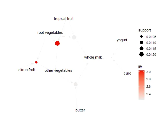
This visualization helps illustrate the strongest associations between items, showing potential cross-selling opportunities or insights into customer behavior:

Each circle (node) represents a different item, and the lines (edges) between them show which items are frequently bought together. The size of each node is the item’s ‘support’, indicating how often the item appears in transactions. The color intensity is the ‘lift’, showing how much more likely items are to be bought together than both individually by chance.

For example, there is a connection between ‘root vegetables’ and ‘other vegetables’. The strong color intensity indicates a high lift between these items. This shows that customers who buy ‘root vegetables’ are very likely to buy ‘other vegetables’ in the same shopping trip.

A Dimensionality Reduction Example: Principal Component Analysis (PCA)

In this example of dimensionality reduction, we will conduct Principal Component Analysis (PCA) using the wine dataset from the rattle package. PCA is a powerful technique for reducing the dimensionality of a dataset while preserving as much variability as possible.

Loading and Preparing the Data

First, we need to load the dataset and prepare it for PCA. We’ll remove any non-numeric columns and scale the data to ensure that all variables contribute equally to the analysis:

Performing PCA

Next, we perform PCA on the scaled dataset using the prcomp function. The center = TRUE and scale. = TRUE arguments ensure that the data is centered and scaled before performing PCA:

The summary of PCA results provides the standard deviation, proportion of variance, and cumulative proportion for each principal component:

	Standard_Deviation	Proportion_of_Variance	Cumulative_Proportion
PC1	2.1693	0.3620	0.3620
PC2	1.5802	0.1921	0.5541
PC3	1.2025	0.1112	0.6653
PC4	0.9586	0.0707	0.7360
PC5	0.9237	0.0656	0.8016
PC6	0.8010	0.0494	0.8510
PC7	0.7423	0.0424	0.8934
PC8	0.5903	0.0268	0.9202
PC9	0.5375	0.0222	0.9424
PC10	0.5009	0.0193	0.9617
PC11	0.4752	0.0174	0.9791
PC12	0.4108	0.0130	0.9920
PC13	0.3215	0.0080	1.0000

• Each PC is a new variable that is a linear combination of the original variables. PCs are ordered by the amount of variance they capture from the data. PC1 captures the most variance, followed by PC2, and so on.
• There are 13 PCs because the original dataset has 13 numeric variables.
• By selecting a subset of the principal components that capture the majority of the variance (e.g., the first few PCs), we can reduce the dataset’s dimensionality from 13 variables to a smaller number, making it easier to visualize and analyze.

Analyzing the Results

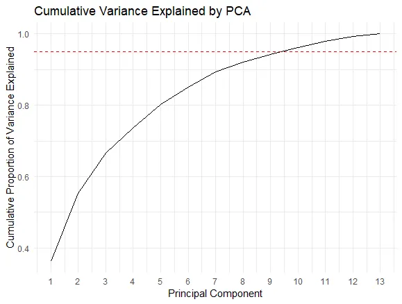
Let’s visualize the PCA results to see how much variance is captured by each principal component:

The plot shows the cumulative variance explained by the principal components. The goal is to choose the number of principal components that capture a high proportion of the variance, typically around 95%:

Based on the plot, we can see that the first 10 principal components capture more than 95% of the total variance. Therefore, we would choose these 10 components to effectively reduce the dimensionality of the dataset while retaining most of the variability. In conclusion, we reduced dimensionality of this data: we went from 13 to 10 components while still capturing over 95% of the variance in the data.

Summary

Additional Resources

• Want to learn more on how to implement these methods and others? Check out this article and this course on Datacamp if you are using R.
• Do you prefer learning how to do unsupervised learning in Python? Check out this course on Datacamp.