


Overview
This article is a follow-up to Get Introduced to Machine Learning, which covered the basics of different machine learning types. In this article, we will dive deeper into one of the types of machine learning: Supervised Learning.
This in-depth introduction to supervised learning will cover its key concepts, algorithms and provide hands-on examples in R to illustrate how you can use these concepts in practice. Whether you are new to this topic, only have basic coding skills or just curious about supervised learning - this article will equip you with the tools to start your first supervised learning model.
The article covers several topics:
- What is Supervised Learning?
- Supervised Learning Algorithms
- A Regression Example
- A Classification Example
What is Supervised Learning?
Supervised Learning involves training a model on a labeled dataset, which means that each observation (e.g., customer) in the training sample is "tagged" with a particular outcome (e.g., "buy"). The model learns by comparing its own predicted output with the true labels that are given, and adjusts itself to minimize errors. By doing this, it improves its prediction abilities over time, with the goal of accurately generalizing previously unknown data.
There are two types of algorithms:
- Regression
- Classification
With regression, the model predicts continuous or numerical values such as the weather, housing prices, or profit. The goal is to estimate the relationship between independent variables (features) and the dependent variable (target).
Classification, on the other hand, is used for categorical output variables. It assigns data into two or more classes, such as customer retention or churn, identifying emails as spam or not, or recognizing handwritten text. The goal is to correctly classify new input data in their corresponding categories.
Key Concepts
- Labeled Data: in supervised learning, the model is trained with labeled data. This means that the target for this data is already known. These predefined tags help the model to develop and learn on its own, so that it is able to predict targets more accurately when given new unseen and unlabeled data.
- Features: input variables are called features. These are independent variables that describe your data, and are used to predict or explain the target variable.
- Target: output variables are called targets. This is the dependent variable that the machine is trying to predict or understand.
- Data split: to train the model, data is usually splitted into a training and testing sample. This is done to prevent overfitting, meaning that the model works very well on the training data, but could possibly not generalize to new unseen data. As an example, we can use 80% of the data as input to the model to learn from, and use the other 20% to validate how well the model works on new input. Keep in mind that even though in most cases it is good practice to use a train-test split, it is not always necessary or suitable for your model.
Supervised Learning Algorithms
There are many different algorithms you can use in supervised learning. Here are some examples:
- Linear Regression:
Used for regression tasks, this algorithm models the relationship between the features and target as a linear equation. It shows trends and estimates the values of the slope and the intercept based on labeled training data. An example is predicting house prices, with features such as the neighborhood and the number of bedrooms.
 Warning
Linear regression assumes a linear relationship between variables. However, in real life, this assumption may not always hold. This algorithm is maybe not suitable if you need to capture complex non-linear relationships between variables.
- Logistic Regression:
Logistic regression is used for binary classification. This means it can model only two possible outcomes, such as yes/no, 0/1, or true/false. Instead of exactly classifying an outcome, it gives the probability between 0 and 1 that an outcome is in one of two classes. This method is easy to implement and understand. An example is predicting if a football team will win a match or not.
- K-Nearest Neighbors (KNN):
KNN can be used for both regression and classification. It calculates the distance between data points, and bundles points together into a group that are near to each other. It predicts the output based on the majority vote (for classification) or the average (for regression) of the "k" number of nearest neighbors.
WarningIt is important to select the k that suits your data. A small value of k means that noise will have a higher influence on the result, whereas a large value makes the algorithm slower and may also make it too general. The best value of k is usually found through cross-validation.
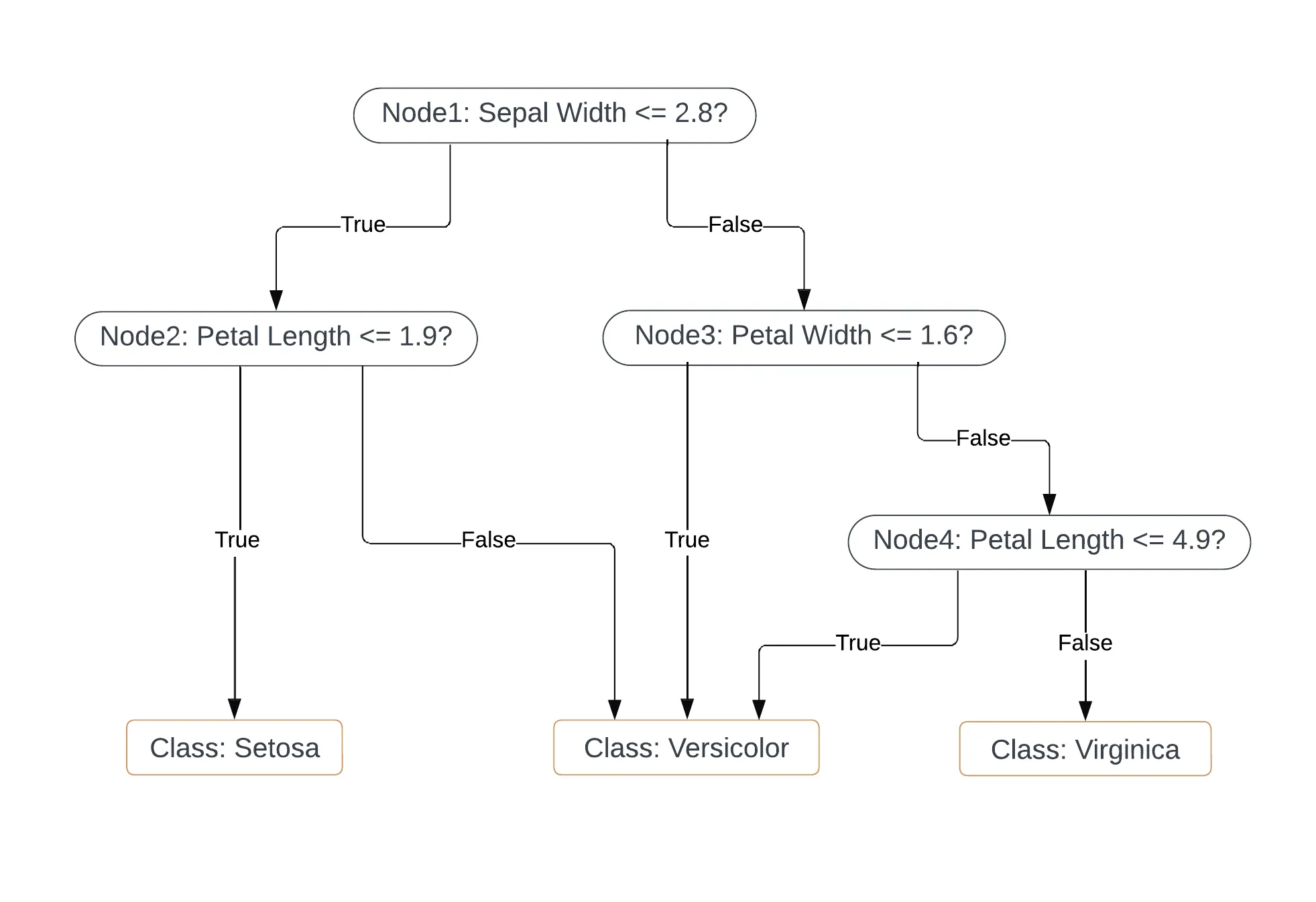
- Decision Trees:
Decision trees can be used for both classification and regression, and is often used because it is a visually interpretable model. It builds a tree where each so-called "node" splits the data based on a simple decision rule. Each "branch" then splits the data on the outcome of this rule. The deeper the tree, the more complex these decision rules get. Below is an example of a decision tree that classifies flowers in one of three species with four input features.
 Tip
TipDecision trees are great for visual interpretability. However, due to their high variance, they tend to perform worse in terms of predictability. To reduce this variance and to make better predictions, you can use Random Forests.
- Random Forests:
Random forests is an ensemble method that builds multiple decision trees to improve prediction accuracy and control overfitting. Random forests average many decision trees to reduce their inherent high variance. Read more in this Introduction to Random Forests in Python.
- Support Vector Machines (SVM)
SVM is a powerful algorithm for classification problems. It identifies a line called a "hyperplane" that separates different categories. The algorithm's objective is to place this hyperplane in such a way that the gap between the closest points of different classes on either side of the line is maximized. An example of SVM is face detection, where the algorithm classifies parts of an image as a face or non-face and recognizes different facial expressions.
- Neural Networks
Neural Networks are inspired by the structure and function of the brain's neural networks and are powerful in modeling complex patterns. They consist of layers of nodes, or "neurons," that make simple calculations from their input. The data goes through an input layer, then through one or more "hidden" layers, and finally through an output layer. Neural networks are particularly effective for complex problems. An example is image recognition, where a neural network can identify and classify objects within images.
WarningNeural networks act as "black boxes," making it difficult to understand the exact nature of the decision-making processes. Furthermore, it can be very computationally intensive to train a neural network. Other algorithms might achieve similar results with greater efficiency.
A Regression Example: Linear Regression
In this example of supervised regression in R we will predict someone's weight based on their height, using a dataset provided by the datasets package. We will use a simple linear regression model.
Loading and Inspecting the Data
First, load the women dataset and inspect what it looks like:

# Load the data as df
library(datasets)
data(women)
df <- women # call the dataframe `df`

# Inspect the data
summary(df)
plot(df)
This data contains two columns. One for the height and one for the weight. There are 15 observations.
Splitting the data
We will split the dataset into a training and a testing set. The training set is used to train the model, and the testing set is used to evaluate its performance later.
We specify how large we want the split to be, and randomly assign rows to one of two dataframes df_train or df_test:
# Splitting the data
set.seed(123)
N <- nrow(df) # Number of rows in df
training_rows <- sample(1:N, 0.75*N) # 75-25 random split

df_train <- df[training_rows, ] # Training data
df_test <- df[-training_rows, ] # Testing data

# Verify the number of rows
nrow(df_train)
nrow(df_test)
Always set the seed with set.seed(123) before you start building any model. This ensures reproducibility. You can choose any number inside the brackets: the seed itself carries no inherent meaning.
Training the Model
We will use a simple linear regression to predict weight based on height. weight is the target and height the feature. We only use the training data in df_train:
# Train the model
model <- lm(weight ~ height, data = df_train)
If you use multiple features, you can use the following command to include all independent variables in the regression:
lm(weight ~ ., data = df_train)
Making Predictions
After training the model, we will make predictions using the df_test data.
These predictions are added to a new column in the testing dataframe called weight_pred.
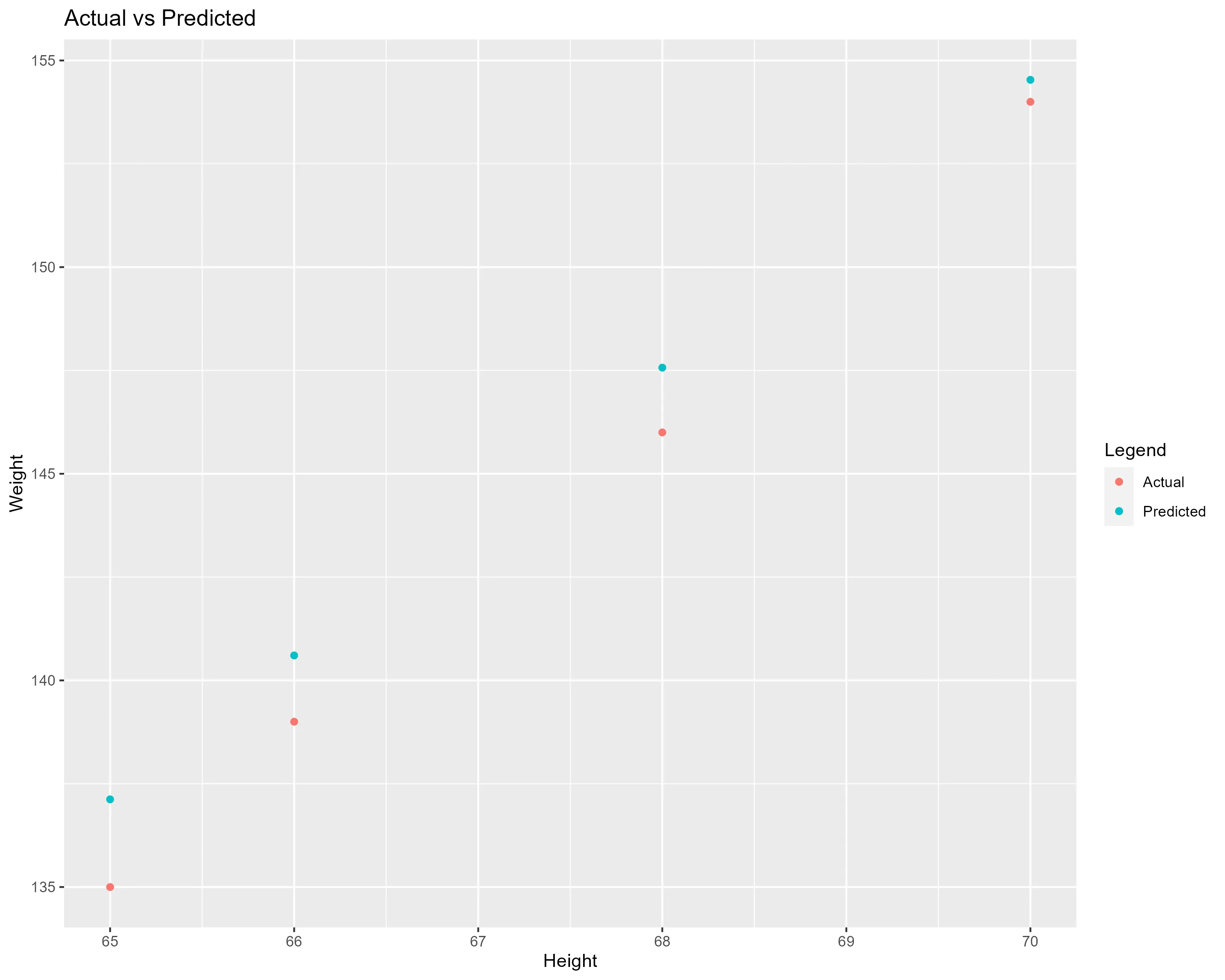
After, we inspect the results by printing and plotting the predictions against the actual values in weight:
# Predict values and assign to new column `weight_pred`
df_test$weight_pred <- predict(model, newdata = df_test)

# Print and plot the results
df_test[c("weight", "weight_pred")]

# install.packages("ggplot2") # Uncomment if 'ggplot2' is not installed
library(ggplot2)

ggplot(data = df_test) +
  geom_point(aes(x = height, y = weight, colour = "Actual")) +
  geom_point(aes(x = height, y = weight_pred, colour = "Predicted")) +
  labs(title = "Actual vs Predicted", x = "Height", y = "Weight", colour = "Legend")
Evaluating the Model
Now that we have trained and tested the model, we want to know how well it performs:
# Evaluate the model
# install.packages("Metrics") # Uncomment if 'Metrics' is not installed
library(Metrics)

r_squared <- summary(model)$r.squared
rmse_value <- rmse(df_test$weight, df_test$weight_pred)
Two evaluation metrics for regression are R-squared and RMSE. This is what they mean:
- R-squared: the percentage of the target variance that the model of explains. Higher values (closer to 1) mean that the model accurately captures the outcomes in the training data.
- Root Mean Squared Error (RMSE): the average difference between the predicted and actual values. Lower values mean that the model on average predicts closer to the actual values.
A Classification Example: Decision Trees
In this example of supervised classification in R we will use the iris dataset. This dataset consists of measurements for iris flowers from three different species. We will train a model that can classify the irises into one of the three species. We will do this by making a decision tree.
Loading and Inspecting the Data
First, load the iris dataset and inspect what it looks like:
# Load the iris dataset
library(datasets)
data("iris")
df <- iris # call the dataframe `df`

# Inspect the data
summary(df)
plot(df)
This data contains five columns with flower measurements. There are observations of 150 flowers.
Splitting the data
For classification, we also split the data into a training set and a testing set. We again specify how large we want the split to be, and randomly assign rows to one of the two dataframes df_train or df_test:
# Splitting the data
set.seed(123)
N <- nrow(df) # Number of rows in df
training_rows <- sample(1:N, 0.80*N) # 80-20 random split

df_train <- df[training_rows, ] # Training data
df_test <- df[-training_rows, ] # Testing data

# Verify the number of rows
nrow(df_train)
nrow(df_test)
Training the Model
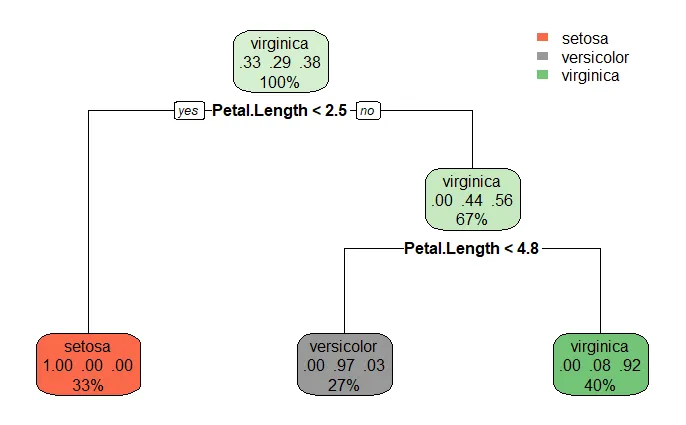
We will use a decision tree to classify flowers in one of three species. Species is the target and all other columns . are the features.
We only use the training data in df_train:
# install.packages("rpart") # Uncomment if 'rpart' is not installed
library(rpart)

# Train the model
model <- rpart(Species ~ ., data = df_train, method = "class")

# Visualize the decision tree
# install.packages("rpart.plot") # Uncomment if 'rpart.plot' is not installed
library(rpart.plot)
rpart.plot(model)
TipIf you are using decision trees for a regression problem, you should adapt the method to "anova":
model <- rpart(Y ~ ., data = df_train, method = "anova")
Making Predictions
After training the model, we will make predictions using the df_test data. These values are assigned to a new column in the testing dataframe called Species_pred. After, we inspect the results by printing the predictions against the actual values in Species:
# Predict values and assign to new column `Species_pred`
df_test$Species_pred <- predict(model, newdata = df_test, type = "class")

# Print the results
df_test[c("Species", "Species_pred")]
Evaluating the Model
Now that we have trained and tested the model, we want to know how well it performs. We look at the confusion matrix, which shows how many observations of each category are correctly classified:
# Evaluate the model
# install.packages("caret") # Uncomment if 'caret' is not installed
library(caret)

confusionMatrix(df_test$Species_pred, df_test$Species)
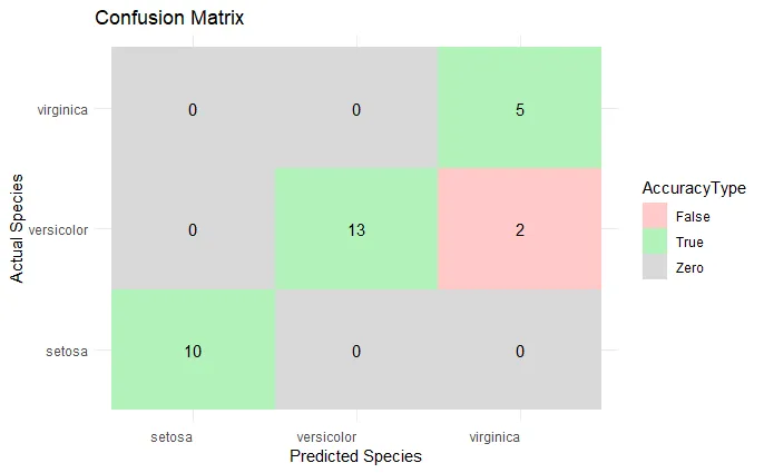
TipFrom the Confusion Matrix you can calculate evaluation metrics like accuracy, precision, and recall.
- Accuracy: the fraction of predictions our model got right, including both true positives and true negatives
- Precision: out of all the instances we predicted as positive (true positives + false positives), how many are actually positive (true positives)
- Recall: out of all the actual positive instances (true positives + false negatives), how many we correctly predicted as positive (true positives)
Summary
 Summary
This article introduced you to Supervised Machine Learning. We explored key concepts, various algorithms for both regression and classification, and demonstrated these concepts with real-life datasets like Women and Iris.
The key takeaways from this article include:
-
Understanding Supervised Learning: Training models on labeled data to predict outcomes on unseen data.
-
Exploration of Algorithms: Insight into algorithms like Linear Regression, Logistic Regression, K-Nearest Neighbors, Decision Trees, Random Forests, Support Vector Machines, and Neural Networks.
-
Practical Applications: Step-by-step examples in R using the Women dataset for regression and the Iris dataset for classification, from data loading and model training to prediction and evaluation.
-
Model Evaluation: Learned about evaluation metrics such as the R-squared, RMSE, confusion matrices, accuracy, precision, and recall to understand model performance.
Additional Resources
- Want to learn more on how to implement these methods and others? Check out this article and this track on Datacamp if you are using R.
- Do you prefer learning how to do supervised learning in Python? Check out this skill track on Datacamp.