Introduction
Regression discontinuity (RD) designs are a popular method for causal inference in non-experimental contexts in economics and other fields, such as political science and healthcare. They rely on the existence of a threshold defined as a value of some running variable, to one side of which subjects are treated, and to the other not. Regression discontinuity in time (RDiT) designs are those RD applications where time is the running variable. The cutoff consequently is the treatment date: after it, subjects are treated, and before it, they are not.
The RDiT design is thus useful in cases where there is no cross-sectional variation in treatment status; that is, on a certain date, treatment is applied to all subjects, meaning designs such as difference-in-differences (DiD) are not applicable. Like in canonical (continuity-based) RD designs, in RDiT we identify the treatment effect as a discontinuity in the outcome variable at the cutoff, assuming that any potential time-varying confounders change smoothly around the threshold. However, there are also important differences between standard RD and RDiT designs which have implications for causal inference.
Differences between standard RDD and RDiT
First, in RDiT it is often the case that we only have one observation per unit of time, unlike in many other applications of RDD with a discrete running variable. This happens, for example, with hourly pollution data in environmental economics, a field where RDiT designs are frequently used. In these cases, in order to attain sufficient sample size, researchers often use very wide bandwidths, of up to 8-10 years. In such large time periods, many changes unrelated to treatment are likely to affect the outcome variable. This could be caused by time-varying confounders (in the pollution example, think of weather or fuel prices) or simply time trends in the outcome. Using a long time period after the treatment date can also result in us capturing treatment effects that vary over time, a circumstance RD designs are unsuited to.
In addition, if our time variable is measured sparsely, i.e. at low-frequency units like months or quarters, the usual assumptions of smoothness and continuity of the conditional expectation function relating the running variable to the outcome (and potential confounders) are a priori less likely to hold. Intuitively, almost any variable is less likely to vary smoothly from month to month than from week to week, for example.
Secondly, as time is the running variable, the data will have time series properties. This can translate into two issues: autoregression in the outcome variable (i.e. the outcome depends on its previous values) and serial correlation in the residuals of our fitted RD models (i.e. residuals from observations next to each other are not independent of each other, violating the Gauss-Markov assumptions).
The third difference is that we cannot interpret an RDiT design with the local randomisation approach, because we cannot perceive time as being assigned randomly in a bandwidth around a threshold. Instead, we can only use the continuity-based approach to RD designs in an RDiT setting, using discontinuities in the outcome at the cutoff to identify causal treatment effects.
Finally, as time has a uniform density, it is impossible to conduct standard density tests (such as the McCrary test) for manipulation of the running variable in RDiT designs. This makes it impossible to test for selection into treatment in the form of anticipation, sorting, or avoidance, all of which could bias the treatment estimates.
Potential sources of bias in RDiT designs
The differences mentioned above can result in some degree of bias which threatens causal inference in RDiT designs:
-
Extending the bandwidth: this means we include observations far away from the treatment date, so our regressions pick up time trends and potentially time-varying treatment effects. If we do not account for time trends, we risk them affecting and biasing our treatment effect estimates. In the case of time-varying treatment effects, our regression to the right of the cutoff (i.e. post-treatment) will be computed based on some weighted average of short- and long-run treatment effects. If these are significantly different, we will estimate a different discontinuity than if we had been able to focus on short-run effects, leading to bias in the treatment estimates. In addition, significant differences between short- and long-run treatment effects may cause our global polynomial to overfit.
-
Time-varying confounders: the basic assumption in a continuity-based RD design is that any potential confounders change continuously around the threshold. This is less likely to hold if we measure time at low-frequency, wide intervals like months. If confounders change discontinuously around the treatment date, we will be estimating biased results which include both the true treatment effect and selection bias.
-
Serial correlation in residuals: if this is present, our conventional standard errors will be incorrect. This threatens causal inference by invalidating our confidence intervals and calculations of statistical significance.
-
Autoregression in the outcome variable: if the outcome variable is dependent on its previous values and this is not accounted for, our treatment effect estimates will include both the true treatment effect and the autoregressive effect of lagged values on present values. Also, autoregression may cause global polynomials to overfit, as in the case of time-varying treatment effects. It is important to note that this is more likely to occur when time is measured at high-frequency levels.
-
Manipulation of the running variable (selection into treatment): in an RDiT context, this can take the form of sorting, anticipation, or avoidance. For example, subjects anticipate the introduction of tougher regulation on installing polluting facilities and move forward their installation to just before the treatment date. This can also happen in canonical RDDs, but in RDiT designs it represents a bigger problem because we cannot formally test for such behaviour. Hence, any effects we estimate will be composed of both the true treatment effect and manipulation-related effects, if any.
Recommendations for RDiTs in practice
Given this susceptibility of RDiT designs to bias, Hausman and Rapson (2018) provide several recommendations to improve the credibility of causal inference in these settings:
-
To informally check for time-varying treatment effects, plot the residuals of a regression of the outcome on any relevant covariates (not including the treatment dummy in the regression) against time. Use various specifications of the time trend (at least linear and quadratic). If the residual plots with different time trends are substantially different, this may indicate the presence of time-varying effects. If the residuals appear to exhibit seasonal or cyclical patterns, consider including time/season fixed effects in your regression.
-
Conduct standard tests for sensitivity to polynomial order and bandwidth choice.
-
Conduct placebo RD estimations on fake treatment dates and, if applicable, nearby geographic areas not subject to the treatment.
-
Plot the relationship between time and any potential confounders to demonstrate continuity at the cutoff. Additionally, regress each potential confounder on the treatment to provide more formal proof of continuity. If there are discontinuities, include covariates capturing these time-varying confounders in your regression.
-
Estimate a ‘donut’ RD, removing observations just before and after the treatment date, to minimise the threat to inference from any sorting, anticipation, or avoidance effects, which are likely to be concentrated in the period right around the treatment date. This will help to allay doubts about the possibility of manipulation/selection into treatment in biasing our estimates.
Tip
'Donut' regression discontinuity designs are frequently used when there is non-random 'heaping' in the data. Heaping refers to cases where certain values of the running variable have much higher densities than adjacent values. This is often the case when there is some type of manipulation of the running variable: think of the pollution example - if polluters realise that a new regulation will be enforced on day $x$ (they anticipate the policy), they might want to install their polluting facilities on day $x-1$. If many of them do so simultaneously, we will observe much higher values of installations on day $x-1$ than on nearby dates. Barreca et al. (2011) show that estimating regular RD regressions when there is such non-random heaping yields biased estimates. Intuitively, the presence of such 'heaps' violates the smoothness assumptions which are essential for RDDs to give unbiased treatment effect estimates. Donut RDDs solve this problem by simply dropping all observations at the 'heaps' and re-estimating the regressions without these observations. Barreca et al. (2011) show that this is the most robust way of estimating unbiased treatment effects in RD settings with manipulation/heaping. Therefore, it is good practice to use the donut RDD approach, i.e., dropping observations around the cutoff, where heaping is most likely to occur in RDiT settings, as a robustness check in RDiT designs where we suspect (remember that we cannot explicitly test for manipulation when time is the running variable) manipulation/heaping is present.
-
Test for serial correlation in residuals, for instance using a Durbin-Watson test. If serial correlation is present, compute heteroskedasticity and autocorrelation consistent (HAC) standard errors, also known as Newey-West standard errors. In some applications it may also be relevant to test for autoregression in the outcome variable and include lagged values of the outcome variable if autoregression is indeed present.
-
To avoid using an excessively wide bandwidth, estimate treatment effects using Hausman and Rapson’s (2018) ‘augmented local linear’ methodology. In the first stage, use the full data sample to regress the outcome on covariates/potential confounders only, excluding the treatment variable. In the second stage, regress the residuals of the first stage on the treatment, using an appropriate narrow bandwidth. See section 3 of Hausman & Rapson (2018) for further reference.
Tip
For more information on sensitivity and placebo tests (points 2, 3, and 4), as well as validation and falsification analysis for RDD more generally, see this topic.
Estimating RDiT in R
Now we apply some of the recommendations described above to a dataset used in González (2013), who uses RDiT to estimate the effect of a universal child benefit in Spain on fertility, abortions, and mothers’ labour supply. The covariate-related recommendations cannot be applied in this case because the dataset does not include any relevant covariates.
First, we load the necessary packages and the data, which is available on surfdrive in STATA 11/12 format.
#load packages
library(foreign) #to read data in STATA format
library(tidyverse)
library(rdrobust) #for plots
library(lmtest) #to run a Durbin-Watson test
library(sandwich) #to compute HAC standard errors
#load the data
theUrl_ca4b <- "https://surfdrive.surf.nl/files/index.php/s/JAo4jnvf042xQXt/download"
fertility <- read.dta(file = theUrl_ca4b)
#sort the data by date
fertility <- fertility[order(fertility$date),]
Before running our RDiT regressions, we can make a plot to visualise the data and the potential discontinuity at the treatment date. We focus on the abortions outcome variable. Note that the treatment (the child benefit) was introduced in July 2007 (this is coded as date=570 in the dataset) and that time is measured at the monthly level. Therefore, the time variable is centred on July 2007. In this case, we use a second-order polynomial (a quadratic), but you could also experiment with other polynomials by changing p in the function below. We also select a 36-month (3-year) bandwidth, and you could also try experimenting with that (in the paper, effect estimates are robust to bandwidth choice).
#use the with function to select a bandwidth
#set polynomial order with p=...
#set number of bins with nbins=...
#y.lim is used to define the height of the y-axis
with(subset(fertility, date >= 540 & date <=599), rdplot(y = abortions, p=2, x = month_of_conception, nbins=30, y.lim = c(0, 10000), title="Discontinuity in abortions after the introduction of the benefit", x.label="Month (centered on policy introduction date)", y.label="Abortions"))
Output
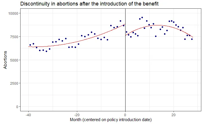
We see a clear discontinuity at the treatment date. Now, we can test for this formally by running a standard RDiT regression:
#estimation of treatment effect with a second-order polynomial
#use natural log of abortions as in the paper
options(scipen = 999) #remove scientific notation
fertility$month_qdr <- fertility$month_of_birth^2 #create quadratic of the time variable
rdit <- lm(ln_abortions ~ month_of_birth + month_qdr + treatment_dummy + month_of_birth*treatment_dummy + month_qdr*treatment_dummy, subset(fertility, date <= 599 & date >= 540))
summary(rdit)
Output
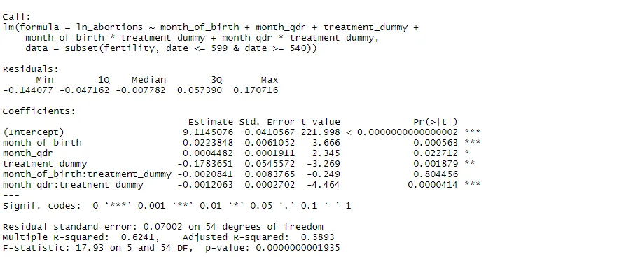
We see a statistically significant negative effect of the treatment on abortions, which is also what Gonzalez (2013) finds in her paper. Now, let's run some of the robustness checks mentioned above. We start by testing for serial correlation in the residuals using the Durbin-Watson test.
Output

We see that the p-value is well below 0.05, meaning we can reject the null hypothesis of no serial correlation. Given that residuals exhibit this serial correlation, we compute HAC standard errors:
#use vcovHAC in coeftest to re-estimate the model with HAC standard errors
coeftest(rdit, vcovHAC(rdit))
Output

The HAC standard errors do differ from the conventional ones, but do not change the inference we made from the original estimates. The treatment coefficient remains strongly statistically significant.
Now, we estimate a donut RDD, allowing for the possibility that individuals anticipate the policy and change their behaviour accordingly. We assume that they can do so within 1 month of the treatment date (before and after).
#donut RDD removing 1 month before and 1 month after the treatment date
rdit_donut <- lm(ln_abortions ~ month_of_birth + month_qdr + treatment_dummy + month_of_birth*treatment_dummy + month_qdr*treatment_dummy, subset(fertility, date <= 599 & date >= 571 | date <= 568 & date >= 540))
summary(rdit_donut)
Output
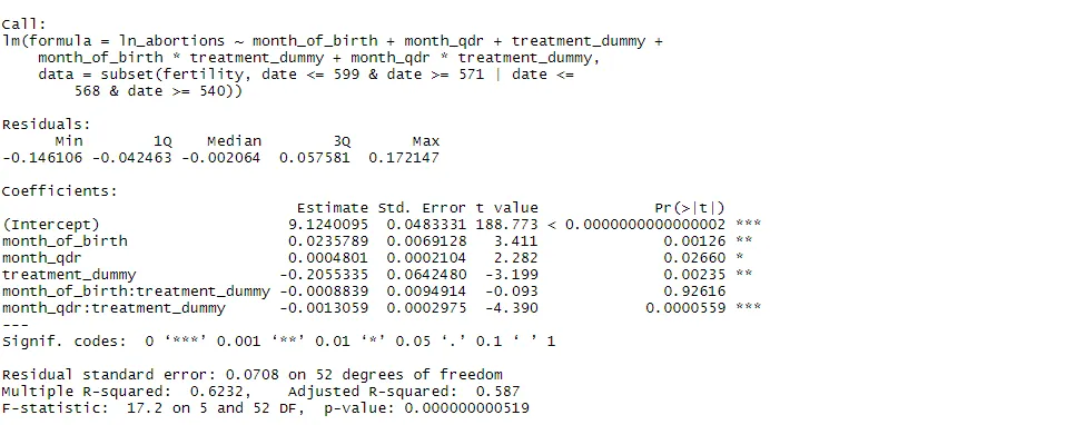
Again, the coefficient estimates remain significant after we remove observations just below and after the cutoff. The model is robust to potential manipulation effects. Finally, we perform a placebo test, running the same RDiT regression on a fake treatment date, which I choose to be July 2004 (coded as 534 in the dataset). We uses the same bandwidth (36 months to either side). We can first plot this placebo discontinuity to visualise it:
#create variables to estimate placebo RDiT
fertility$fake <- ifelse(fertility$date >= 534, 1, 0) #dummy for fake treatment
fertility$fake_month <- fertility$date - 534 #center time on the fake treatment date (July 2004)
fertility$fake_qdr <- fertility$fake_month^2 #quadratic of time centred on the fake treatment date
#plot the placebo discontinuity
with(subset(fertility, date >= 497 & date <=569), rdplot(y = abortions, p=2, x = fake_month, nbins=30, y.lim = c(0, 10000), title="Discontinuity in abortions at the fake treatment date", x.label="Month (centered on fake policy introduction date)", y.label="Abortions"))
Output
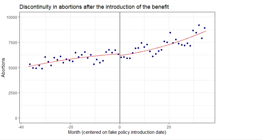
We can already see that there is not much of a discontinuity at the fake treatment date. We now test this formally:
placebo <- lm(ln_abortions ~ fake_month + fake_qdr + fake + fake*fake_month + fake*fake_qdr, subset(fertility, date <= 569 & date >= 497))
summary(placebo)
Output
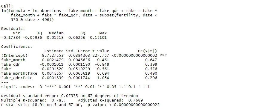
The regression results confirm that there is no significant discontinuity in the outcome at the fake treatment date. The model has therefore passed all of our robustness checks. In many applications, it would also be useful to conduct further checks related to time-varying confounders, but this is not possible here because the dataset does not include any relevant covariates.
Summary
We can use regression discontinuity in time (RDiT) designs when the treatment we are interested in is implemented at a certain date and is applied to all subjects, meaning we have no cross-sectional control group. However, we must be aware of the shortcomings and potential sources of bias inherent in RDiTs, namely using very wide bandwidths to generate sufficient sample size, serial correlation and autoregression, and manipulation. The table below provides a summary of the robustness checks we can use to mitigate concerns about these biases:
| Bias | Solution |
|---|---|
| Discontinuously time-varying confounders | Regress outcome on covariates to test for discontinuities; control for confounders in the regression if necessary |
| Excessively wide bandwidth: time-varying treatment effects | Plot residuals with different specifications of time trends to visualise time-varying effects; Augmented local linear procedure of Hausman & Rapson (2018) |
| Excessively wide bandwidth: time trends | Placebo tests on fake treatment dates, time/season fixed effects, various polynomials to model time-outcome relationship |
| Serial correlation in residuals | HAC/Newey-West standard errors |
| Autoregression in the outcome variable | Lagged values of the outcome in the regression |
| Manipulation | Donut RDD |


