Introduction

This topic discusses causal inference from regression discontinuity designs (RDDs) where the running variable determining treatment assignment is discrete. This is a practically relevant application of RDDs, given that treatments are often assigned based on discrete variables such as age, date of birth, or calendar time.

RDDs are applied in settings where treatment probability changes discontinuously around a certain cutoff or threshold. This cutoff refers to a value of the running variable (also known as the assignment variable or the score) based on which a certain policy or treatment is applied or assigned. For example, in the case of the legal drinking age, age is the running variable, and the minimum legal drinking age is the cutoff. RD designs can be sharp, if treatment probability changes from 0% to 100% at the cutoff, or fuzzy, if treatment probability changes less drastically (but still discontinuously) at the cutoff, such as in the case of the legal drinking age.

This topic explains the issues associated with discrete as opposed to continuous running variables and discusses the different approaches used to deal with them.

Approaches to RDD: continuity-based vs local randomisation

Causal inference in RDDs can be based on either the continuity-based or the local randomisation approach. The fundamental assumption of the continuity-based approach is that the observable and unobservable characteristics of subjects change smoothly and continuously around the cutoff point, allowing us to infer that any discontinuous differences in the outcome of interest at the cutoff are the result of differences in treatment assignment. The treatment effect given by such methods is the treatment effect at the cutoff, equivalent to the ‘jump’ or discontinuity observed graphically.

The local randomisation approach rests on the assumption that, for observations sufficiently close to the cutoff, treatment is as good as randomly assigned, akin to a randomised experiment. This implicitly relies on the idea that subjects just below and just above the cutoff have roughly equal chances of being in the treatment and control groups. For canonical RDD applications with continuous running variables, the assumptions of local randomisation are stronger than those for the continuity-based approach and, as such, the latter is commonly preferred in such cases.

The problem of discrete running variables

If the running variable is discrete, however, this need not be the case. Local polynomial methods process each distinct value of the discrete running variable (also called a support point or a mass point) as a single observation. If there are many support points which are sufficiently close to each other, the continuity assumption is still plausible and estimation as in continuous running variable RD designs is valid. However, if support points are few and sparse, it is much less likely to be the case that the relevant observable and unobservable characteristics change continuously with the running variable. RDD applications with discrete running variables and few values of these variables are therefore often better suited to the local randomisation approach.

Using local randomisation with few distinct mass points

\( \)

Identification in the local randomisation approach rests on the formal assumption that, within a certain sufficiently narrow bandwidth bounded by $c-h$ and $c+h$, where $c$ is the cutoff value, units just above and just below the cutoff are fundamentally similar and comparable to each other, and that therefore treatment assignment based on the cutoff value is as if random. This implies that the running variable is random and orthogonal to the values of the outcome variable.

The advantage of the local randomisation design when the running variable is discrete is that it does not rely on assumptions about the continuity of the regression functions on either side of the cutoff. This is relevant because when the running variable is discrete and there are large gaps between the mass points, it is often implausible to assume that the conditional expectation function relating the running variable to the outcome is continuous. We are also unable to observe the nature of the CEF within each mass point. For example, if our running variable is income grouped by ranges (e.g., €24,000-€24,999.99, €25,000-€25,999.99 etc.), we can observe values of the outcome for each range, but not for each individual subject within that range. That is, we cannot discern the relationship between income and the outcome for individuals earning between €24,000 and €24.999.99. By lifting the continuity assumptions, the local randomisation approach allows us to study treatment effects in RD designs where the assignment variable is discrete, low-frequency, and sparse.

The main disadvantage of the local randomisation approach is that the assumption that the outcome is independent of the running variable is unlikely to hold in many settings, at least within a reasonable bandwidth. The further an observation is from the cutoff, the less likely it is that it is truly comparable to observations on the other side, and the more likely it is that the outcome for that observation is affected by its value of the running variable. Thus, using the local randomisation approach often requires extremely narrow bandwidths, defining which is sometimes unfeasible. Returning to our earlier example of income ranges, let’s now assume that our mass points are defined as broader ranges: e.g., €20,000-€24,999.99, €25,000-€29,999, etc. Suppose a treatment is applied to individuals with incomes below €25,000. In the previous case we could reasonably assume individuals earning €24,100 and €25,900 are sufficiently comparable, and thus use €24,000 as the lower bound of our bandwidth and €25,999.99 as its upper bound. In this case, due to the wider ranges, we cannot do this. At the same time, it seems much less appropriate to assume that individuals earning €21,000 and €29,000 are sufficiently comparable, thus, we also cannot credibly define €20,000 and €29,999.99 as the lower and upper bounds of our bandwidth.

In cases where the local randomisation approach cannot be applied because of the restrictions it places on bandwidth size, we can use an amended version of the continuity-based approach described by Kolesár and Rothe (2018).

Using the continuity-based approach with ‘honest’ confidence intervals

We’ve already seen why we cannot apply the conventional continuity-based approach to settings where the running variable takes on only a few distinct values. Essentially, it is difficult to credibly ascertain the functional form of our regression equation, leading to specification bias. Of course, some degree of specification bias is always present, because the true form of the CEF is almost never exactly linear or quadratic. However, when the CEF is estimated over a sufficiently narrow bandwidth, the size of this specification bias relative to the standard error of the treatment estimator is negligible and approaches zero. This allows us to use conventional confidence intervals based on (heteroskedasticity-robust) Eicker-Huber-White standard errors (EHW) for causal inference without correcting for specification bias.

In settings where the running variable only takes on a few distinct values, we usually cannot use very narrow bandwidths because this leads to an excessively small sample size. As we expand the bandwidth to gain enough observations for our estimation, specification bias increases. As we consider values further and further away from the cutoff, we are more likely to mis-specify the functional form at the cutoff, biasing our treatment estimates (which in the continuity-based approach are effects at the cutoff). The bias of our treatment estimator becomes larger and non-negligible with respect to its standard error. In this case, we cannot use conventional EHW confidence intervals, because they fail to account for this bias and are therefore too narrow, exacerbating the false positive rate (type I error).

Kolesár and Rothe (2018) show that this issue cannot be solved by clustering standard errors at each value of the discrete running variable, as was previously thought. Instead, they propose two alternative methods for constructing confidence intervals for causal inference in the case of RDDs with few distinct values of the assignment variable. In this topic, we mainly discuss the first approach, which is based on bounding the second derivative of the CEF. This is because it holds more generally than the second approach, based on bounding the misspecification error at the cutoff, which requires stronger conditions to work as an honest confidence interval.

Bounding the second derivative (BSD) confidence intervals

Kolesár and Rothe (2018) use the BSD method to estimate the maximum bias the treatment estimator can suffer from and include this bias in the confidence interval as follows:

\( \)

$$\hat{\tau} \pm (B + cv^(1-\alpha)*\frac{\sigma}{\sqrt{N}})$$

Where $\hat{\tau}$ is the treatment estimator, $B$ is the maximum bias, $cv^(1-\alpha)$ is the critical value at the significance level $\alpha$ that we are interested in, and $\frac{\sigma}{\sqrt{N}}$ is the standard error of the treatment estimate.

The maximum bias of the treatment effect refers to the difference between the real effect and that estimated by specifying the least fitting CEF. Naturally, in order to calculate this, we need to impose some restrictions on what type of function the CEF can be. To do this, we consider a function space $\Mu$ in which the second derivative of each function $\mu(x)$ is bounded (in absolute value) by some constant $K$. This allows us to calculate maximum bias conditional on the choice of K. In practice, we compute this maximum bias using the RDHonest package, available in both R and Stata. Once the maximum bias is computed, we can adjust our confidence intervals (as above) and p-values, using the following formula:

p-value = $\frac{\hat{\tau} - B}{\frac{\sigma}{\sqrt{N}}}$

The resulting BSD confidence interval has the following properties:

• It is honest with respect to the function space $\Mu(K)$.
• It is valid regardless of whether the running variable is discrete or continuous.
• It is valid for any choice of bandwidth.
• It allows the researcher to choose a bandwidth minimising the size of the interval in order to obtain the tightest possible confidence interval without invalidating the results.

Implementing Honest BSD confidence intervals in R

In this section, we demonstrate a simple implementation of BSD confidence intervals in R using the RDHonest package. The package includes some datasets, such as cghs, which relates to Oreopoulos’s (2006) study of the effects of a change in the minimum school leaving age in Britain on earnings. Oreopoulos uses age as the discrete running variable of his study.

Output

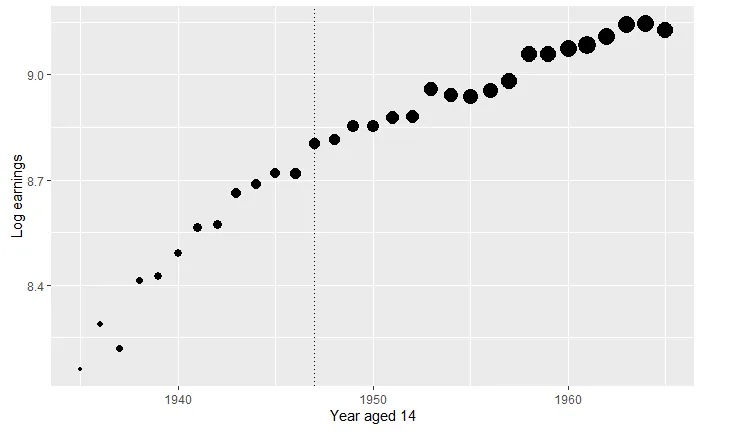
We can first visualise the regression discontinuity by using the RDScatter function built into the package.

Output

Now, we can estimate the treatment effect, the maximum bias, and the corresponding honest confidence intervals using the RDHonest function.

Output

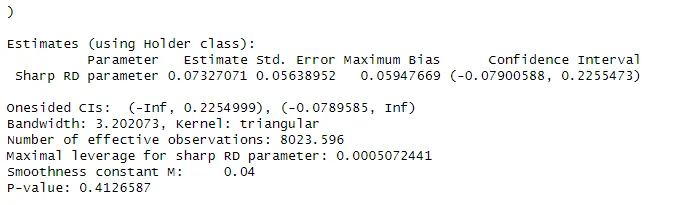
In the regression output we can see the treatment estimate, the maximum bias, and the confidence intervals and p-value computed accounting for this bias.

Summary

Method	Distinct mass points	Bandwidth	Treatment Estimates
Local randomisation	Few and sparse	Narrow	Within window
Conventional continuity	Many and close	Narrow	At cutoff
Continuity with honest confidence intervals	Many and sparse	Wide	At cutoff

See Also

Inference in Regression Discontinuity Designs with a Discrete Running Variable - Kolesár and Rothe (2018)

A Practical Introduction to Regression Discontinuity Designs: Extensions - Cattaneo, Idrobo, and Titiunik (2023)