


Overview
The fixed effects (FE) model, also known as the "Within estimator", captures changes within groups. By focusing on within-group variations, the FE model can control for unobserved entity-specific effects.
When analyzing panel data, it is crucial to account for these unobserved effects to obtain unbiased results. Not controlling for them when they are present in your model, will violate Assumption 1 of the Fixed Effects Regression Assumptions. In other words, the error term will be correlated with the independent variables. This correlation can introduce omitted variable bias.
 Warning
Note that an FE model cannot examine the influence of time-invariant variables on the dependent variable, as these variables are already captured in the fixed effects.
Additionally, a FE model may encounter issues of collinearity when dealing with variables that change little over time. Collinearity arises when independent variables are highly correlated, and if a variable changes very little over time, it becomes highly correlated with the fixed effects in the model. This high collinearity makes it hard to disentangle individual effects of this variable on the dependent variable, potentially leading to unreliable estimates.
Estimation of FE model
Continuing with the same example as the previous building block, the FE model is estimated by removing the fixed effects from the original equation. The original model with fixed effects $\alpha_i$ is represented as:
$Y_{it} = \beta_1 X_{it} + \alpha_i + u_{it}$
To remove the fixed effects from the model, the time-specific means are subtracted from each variable, enabling estimation of changes within firms over time.
Since we assume the unobserved fixed effects $\alpha_{i}$ to be constant, subtracting its mean results in a term of zero. As a result, the fixed effects are eliminated through this transformation, while the time-varying component of the error term $u_{it}$ remains.
Estimation in R
While the plm() function can also be used to estimate a FE model, we recommend using the fixest package. Refer to the fixest article for a comprehensive explanation of this package and its functions.
To estimate a FE model using fixest, use the feols() function and specify the fixed effects variable (firm) within the model formula.

# Load packages & data
library(fixest)
library(AER)
data(Grunfeld)
# Model estimation
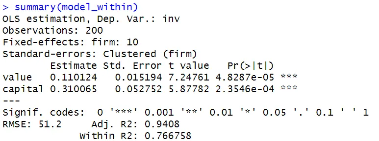
model_within <- feols(invest ~ value + capital | firm,
data = Grunfeld)
summary(model_within)
Time Fixed Effects
Including time fixed effects controls for time trends that are constant across all groups in the panel data and potentially influence the dependent variable. In our analysis of the Grunfeld data set, examples of time trends could be economic cycles, policy changes, or market trends impacting firms' investment decisions.
The model that incorporates both entity-specific and time fixed effects is called a Two-way Fixed Effects model. This model is very commonly used in causal inference analysis.
To include time fixed effects in your model in R, add the variable year to the fixed effects specification:
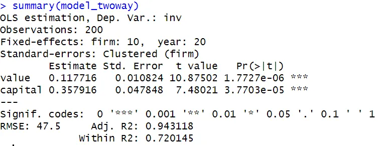
model_twoway <- feols(invest ~ value + capital | firm + year,
                      data = Grunfeld)
summary(model_twoway)
Testing for Fixed Effects: pFtest
To determine whether fixed effects are present in your model, you can use the function pFtest() from the plm package. The pFtest assesses the joint significance of the fixed effects by comparing the FE model to a model without fixed effects, such as the pooled OLS model.
The null hypothesis for the pFtest is that the fixed effects are equal to zero, indicating no unobserved entity-specific effects. The pooled OLS model will be preferred if the null hypothesis is true. The alternative hypothesis is that fixed effects are present in the model. Then, the FE model is preferred over the pooled OLS model.
One disadvantage of the pFtest() function is that it only allows plm objects as arguments. Therefore, we cannot directly use the pFtest() function on the FE model estimated with the fixest package. We estimate the two-way FE model using the plm() function below, to perform the pFtest. We also estimate the pooled OLS model for comparison:
library(plm)

# Estimate the Within model (twoway: Time & Firm FE)
model_within_plm <- plm(invest ~ value + capital,
                    data = Grunfeld,
                    index = c("firm", "year"),
                    model = "within",
                    effect = "twoway")

# Estimate the Pooled OLS model
model_pooled <- plm(invest ~ value + capital,
              data = Grunfeld,
              index = c("firm", "year"),
              model = "pooling")

# Perform the pFtest
pFtest_result <- pFtest(model_within_plm,
                        model_pooled)

print(pFtest_result)
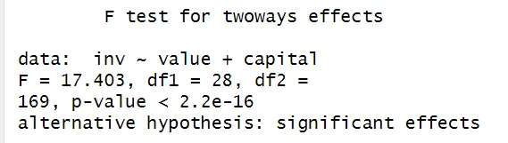
The pFtest result provides the test statistics, its associated p-value, and the degrees of freedom. If the p-value is less than your chosen significance level (e.g., 0.05), you can reject the null hypothesis and conclude that (two-way) fixed effects are present in the model. In this case, the null hypothesis is rejected and therefore the FE model is preferred over the pooled OLS model.
The Least Square Dummy Variable (LSDV) model
Another approach to estimate fixed effects is the Least Square Dummy Variable model. In this model, dummy variables are added for each entity and/or time period to capture the fixed effects. In R, the LSDV model can be implemented using the lm() function and creating dummy variables for the entities and/or time periods.
However, it is important to note that the LSDV approach is not practical for larger panel data sets. When there are many observations (entities and/or time periods), creating dummy variables for each of them can result in a substantial number of variables, leading to computational challenges. Therefore, when dealing with larger data sets, the FE model is preferred as it is a more efficient approach to control for unobserved fixed effects.
 Summary
The FE model, also known as the Within estimator allows us to estimate changes within groups while controlling for unobserved entity-specific fixed effects. By subtracting the time-specific means from each variable, the FE model removes the fixed effects and allows for the estimation of within-group variations over time.
Additionally, the inclusion of time fixed effects accounts for common time trends in the data across groups. The resulting model with both types of fixed effects is called a Two-way fixed effects model and is a widely used approach in causal inference analysis.
In R, the fixest package provides the feols() function for estimating the FE model.
The pFtest() function from the plm package can be used to test for the presence of fixed effects. This can help you decide whether including fixed effects is necessary in your model. However, keep in mind that the pFtest() function requires plm objects as arguments.