


Overview
The Random Effects (RE) model is the last method for panel data analysis discussed in this series of topics. Unlike the Fixed Effects (FE) model, which focuses on within-group variations, the RE model treats the unobserved entity-specific effects as random and uncorrelated with the explanatory variables. After delving into the RE model first, we address probably the most critical choice to make when working with panel data: deciding between an FE or RE model.
This is an overview of the content: - The RE model - Error term structure - Estimation in R - Two-way RE model - Choice between a FE and RE model
The RE model
Let's continue with the model where we estimate the relationship of market and stock value on the gross investment of firms, using Grunfeld data. This is the regression equation:
$invest_{it} = \beta_0 + \beta_1 value_{it} + \beta_2 capital_{it} + \alpha_i + \epsilon_{it}$
where,
- $invest_{it}$ is the gross investment of firm i in year t
- $value_{it}$ is the market value of assets of firm i in year t
- $capital_{it}$ is the stock value of plant and equipment of firm i in year t
- $\alpha_i$ is the fixed effect for firm i
- $\epsilon_{it}$ is the error term, which includes all other unobserved factors that affect investment but are not accounted for by the independent variables or the fixed effects.
The fixed effects $\alpha_i$ represent the time-invariant unobserved heterogeneity that differs across firms. The RE model assumes that $\alpha_i$ is uncorrelated with the explanatory variables, allowing for the inclusion of time-invariant variables such as a person's gender or education level,
Error term in the RE model
The error term (capturing everything unobserved in the model) consists of two components:
- The individual-specific error component: $\alpha_i$.
This captures the unobserved heterogeneity varying across individuals but constant over time. It is assumed to be uncorrelated with the explanatory variables.
- The time-varying error component: $\epsilon_{it}$.
This component accounts for the within-firm variation in gross investment over time. It captures the fluctuations and changes that occur within each firm over different periods. While these time-varying effects can be correlated within the same firm, they are assumed to be uncorrelated across different firms. Note that this correlation of the error term across time is allowed in a FE model as well.
Estimation in R
To estimate the RE model in R, use the plm() function and specify the model type as "random".

# Load packages & data
library(plm)
library(AER)
data(Grunfeld)

# Model estimation
model_random <- plm(invest ~ value + capital,
                    data = Grunfeld,
                    index = c("firm", "year"),
                    model = "random")

summary(model_random)
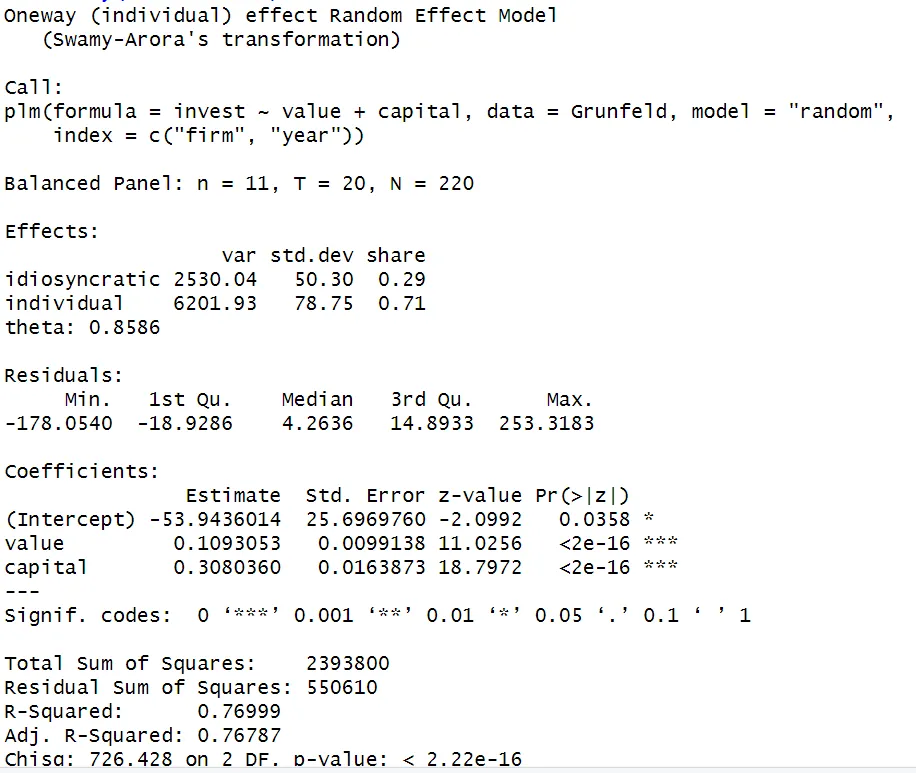
The estimated coefficients capture the average effect of the independent variable (X) on the dependent variable (Y) while accounting for both within-entity and between-entity effects. This means that the coefficients represent the average effect of X on Y when X changes within each entity (e.g., firm) over time and when X varies between different entities.
Two-way Random Effects model
Extend the RE model to a twoway model by including time-specific effects. These time-specific effects are also unobservable and assumed to be uncorrelated with the independent variables, just like the entity-specific effects.
Include effect = "twoways" within the plm() function in R:
# Estimate two-way RE model
model_random_twoway <- plm(invest ~ value + capital,
                    data = Grunfeld,
                    index = c("firm", "year"),
                    model = "random",
                    effect = "twoway")
Choice between Fixed or Random Effects
When deciding between an FE and RE model for panel data analysis, considering the structure of your data is the most important thing to do.
FE model preference
If there is a correlation between unobserved effects and the independent variables, the FE model is preferred as it controls for time-invariant heterogeneity. This is particularly valuable when dealing with observational data where inherent differences among entities (e.g., universities or companies) could affect the outcome.
RE model preference
Opt for the RE model if you are not worried about invariant unobserved effects in the error term. This is often the case in experimental settings where you have control over treatment assignments.
One important reason to use the RE model over the FE model is when you have a specific interest in the coefficients of time-invariant variables. Unlike the FE model, the RE model allows for leaving these time-invariant variables in and estimating their impact on the outcome variable while still accounting for unobserved entity-specific differences.
 Example
Practical example: University performance analysis
Imagine you want to understand if the availability of research grants at universities affects student performance. You have panel data from universities per year, with variables describing their students' performance and research grants. You believe that universities have unobserved university-specific effects, such as its reputation, that could influence both the research grant and student performance but are not included as variables in the data.
Use the FE model - ...if you believe unobserved effects are correlated with grants availability and student performance. You want to control for university-specific factors and isolate grants impact within each university over time. - For example, you suspect that universities with stronger reputations are more likely to secure research grants.
Use the RE model - ...if you believe that unobserved university-specific effects are random and not directly tied to grant availability.
-
RE allows you to add multi-level fixed effects. For example, university-level FE (capturing differences across universities) and student-level FE (capturing differences across students within universities) can be added simultaneously.
-
For example, grant decisions are made by an external committee and largely independent of university-specific characteristics. Moreover, you want to control for both university-level and student-level variations.
| FE Model | RE Model | |
|---|---|---|
| When to Use | Unobserved university- specific effects are correlated with research grants and student performance. | Unobserved effects are random and not directly tied to grant availability. Allows multi-level fixed effects (on university and student-level) in the same model. |
| Example | You believe universities with stronger reputations are more likely to secure research grants. |
Hausman test
To determine the appropriate model, a Hausman test can be conducted to test the endogeneity of the entity-specific effects. - The null hypothesis states no correlation between the independent variables and the entity-specific effects $\alpha_i$. If $H_{0}$ is true, the RE model is preferred. - The alternative hypothesis states a correlation between the independent variables and the entity-specific effects($\alpha_i$). If $H_{0}$ is rejected, the FE model is preferred.
The Hausman test can be performed in R with the phtest() function from the package plm. Specify the FE and RE model as arguments in this function. Note that the models included as arguments should be estimated with plm. Therefore, the Within model is also estimated with plm() first (instead of with feols()from the fixest package like in the Fixed Effects model article).
# Estimate Two-way FE (Within) model
model_within_twoway <- plm(invest ~ value + capital,
                    data = Grunfeld,
                    index = c("firm", "year"),
                    model = "within",
                    effect = "twoway")

# Perform Hausman test
phtest(model_within_twoway,
       model_random_twoway)
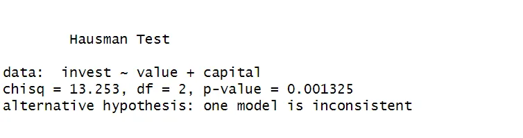
The p-value is 0.0013, which is lower than 0.05. Thus the $H_{0}$ is rejected and an FE model is preferred according to the Hausman test.
Recommended reading
A recommended paper for delving deeper into Random Effects Models is Wooldridge (2019), which introduces strategies for allowing unobserved heterogeneity to be correlated with observed covariates in unbalanced panels.
 Summary
The Random Effects (RE) model is a method for panel data analysis that treats unobserved entity-specific effects as random and uncorrelated with the explanatory variables.
One distinct advantage of the RE model is its flexibility in allowing the inclusion of time-invariant variables, a feature not available in the FE model. Additionally, the RE model allows you to include multi-level fixed effects.
The key difference between the RE and FE model is: - In a FE model, the unobserved effects are assumed to be correlated with the independent variables - In a RE model, the unobserved effects are assumed to be uncorrelated with the independent variables