Overview

This topic will provide an introduction to panel data and how it can be helpful in causal inference analysis. Panel data refers to a specific type of dataset that includes observations on multiple entities over multiple time periods. Unlike pooled cross-sectional data, which can have different cross-sectional units in each time period, panel data follows the same cross-sectional units throughout a given time period.

The growing use of panel data in policy analysis, economics and social sciences can be attributed to its advantageous features. The structure of panel data, analyzing the same cross-sectional units over time, offers several benefits over cross-sectional and pooled cross-sectional data, like:

• Control for unobserved characteristics

Having multiple observations on the same units allows for controlling unobserved characteristics of individuals, firms and other entities. This helps mitigate omitted variable bias and provides more accurate estimates of causal effects.

• Causal inference

The availability of multiple observations in panel data enhances the ability to draw causal inferences. Inferring causality from a single cross-section can be challenging due to potential confounding factors. Panel data allows for analyzing changes within units over time, providing stronger evidence for causal relationships.

• Examination of dynamics

Panel data enables us to examine dynamic processes, such as lagged behavior or the outcomes of decision-making. By observing units over time, changes in variables over different time periods can be understood.

The structure of the article is as follows:

• Introduction to Grunfeld data
• Organising panel data
• Exploring panel data
• Notation of panel data
• Analysis with Grunfeld data
  • Cross-sectional data
  • Unobserved heterogeneity bias
  • Entity fixed effects (data of 2 years)
  • Entity fixed effects (panel data)
  • Entity & Time fixed effects (panel data)

Introduction to Grunfeld data

The Grunfeld data set will be used for an example. It contains investment data for 11 U.S. Firms over a time period of 1935 until 1954. Thus, the data set contains 220 observations (11 firms * 20 years). The following variables are included:

Variables	Description
invest	Gross investment in 1947 dollars
value	Market value as of Dec 31 in 1947 dollars
capital	Stock of plant and equipment in 1947 dollars
firm	- General Motors - US Steel - General Electric - Chrysler - Atlantic Refining - IBM - Union Oil - Westinghouse - Goodyear - Diamond Match - American Steel
year	1935-1954

Load packages and data

Let’s load the necessary packages and the Grunfeld data set:

Organising panel data

The panel data is stored in a two-dimensional way:

• The column firm identifies the entities under observation.
• The column year documents the points in time the data was collected.

A common approach to organize a panel data set is by grouping the data according to the time period of each unit. In this case, the first 20 rows are for the first firm in our data, and each row is for each year (in combination with the first firm). The second 20 rows is for the second firm in our data, and so on. The Grunfeld data set is already structured in this manner, so there’s no need to make any changes here.

To further improve the structure of our panel data set, we rearrange the columns in the following code block. Now, the first column indicates the firm and the second column indicates the year. This enables us to clearly track the temporal aspect of the data.

The function head() returns the first 6 rows of the new Grunfeld data set.

Exploring panel data

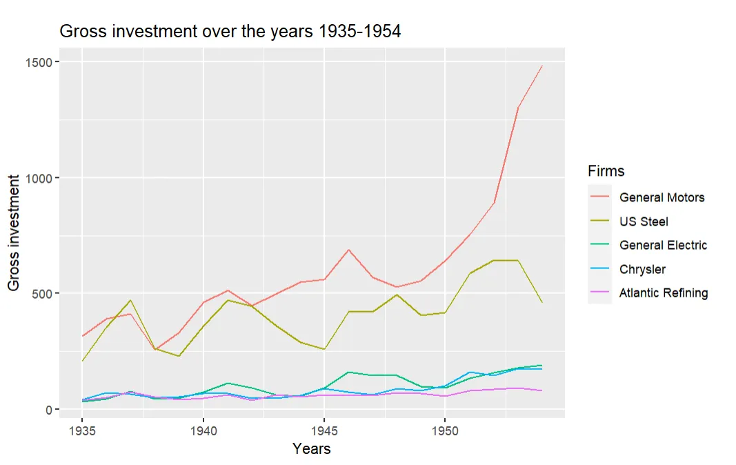
The following plot illustrates the gross investment over the years in the data set, for the first 5 firms in the Grunfeld data set. A subset of 5 firms is chosen to avoid the plot to be too crowded.

Notation of panel data

Panel data typically consists of observations on n entities (such as firms) over T periods (here, years), where $T \ge 2$. Specifically, in the Grunfeld data set, we have information on 11 firms observed across 20 years, resulting in $n = 11$ and $T = 20$.

To represent variables in the dataset, a subscript notation is used, combining the indices for the entity (i) and the period (t). This notation distinguishes a specific observation that corresponds to a particular firm (i) and a given year (t). For example, an observation in the data set is denoted as $Y_{it}$, where $i = 1,…,n$ and $t = 1,…,T$.

Analysis with Grunfeld data

An application of panel data will be done with the Grunfeld data set. Our analysis is about exploring the relationship between market value and gross investment of firms. We start “simple” with cross-sectional and move on to using panel data in steps. Within these steps, the advantages of panel data will become clear!

Cross-sectional data

We start with only cross-sectional data from the year 1935. The variable capital is added as a control variable, and thus the multiple regression model is as follows:

\(invest_{i} = \beta_0 + \beta_1 value_{i} + \beta_2 capital_{i} + \epsilon_{i}\)

where,

• $invest_{i}$ is the gross investment of firm i
• $value_{i}$ is the market value of assets of firm i
• $capital_{i}$ is the stock value of plant and equipment of firm i
• $\epsilon_{i}$ is the error term

The regression equation is estimated using R.

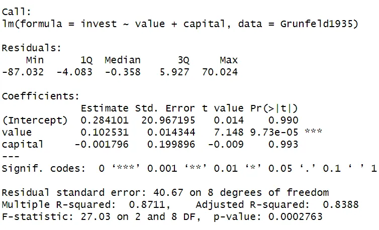
As shown in the summary() of the regression, the coefficient of value is 0.1025 and significant on a 1% level. Thus, this regression using cross-sectional data indicates a positive relationship between the Value and Gross investment of a firm.

Unobserved heterogeneity bias

However, this regression does not tell us much. Using only cross-sectional data may result in omission of variables that influence investment decisions, resulting in biased and incomplete findings. To address this issue, we can include more variables in the equation to control for additional factors impacting gross investment decisions for firms.

However, this approach is not straightforward. Many factors, like firm-specific characteristics, might be unobserved and impossible to control for.

A plot of Firm Value on Gross Investment

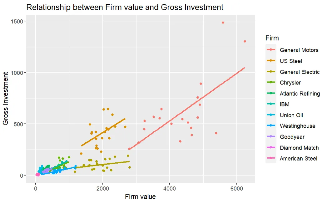
This graph indicates this heterogeneity among the firms. The “starting value” of Gross Investment (without considering the effect of Firm Value) appears to be higher especially for the first two firms, General Motors and US Steel.

To address this heterogeneity, we can use panel data to add firm fixed effects into our model. By doing so, our model will include a specific intercept for each firm, capturing the time-invariant characteristics unique to each firm. This adjustment allows us to control for the heterogeneity observed in the data and provides a more accurate analysis of the relationship between Firm Value and Gross Investment.

There are two types of fixed effects (until now, we only considered the first type):

1. Unobserved effects that are constant over time

In this case, they represent firm-specific characteristics that persistently influence investment behavior. Think of effects like managerial quality, reputation of the firm or the level of risk aversion. For example, a higher managerial quality might result in a higher investment, independent of the firm value.

2. Unobserved effects that vary over time

These time-varying unobserved effects capture factors that change over different periods and affect investment decisions. It allows for the consideration of specific years that may have effects on gross investment unrelated to firm-specific decisions or characteristics. For example, a particular year might experience very bad market conditions, exerting a negative influence on the gross investment of all firms in the data set.

Entity fixed effects (with data of 2 years)

Let’s first consider a data set with 2 time periods, specifically the years 1935 and 1940. Our objective is to eliminate firm-specific effects that remain constant over time, represented by the variable $\alpha_{i}$. We can achieve this by taking the difference between the observations in 1940 and 1935.

The multiple regression model is as follows:

\(invest_{it} = \beta_0 + \beta_1 value_{it} + \beta_2 capital_{it} + \beta_3 \alpha_{i} + u_{it}\)

where:

• $invest_{it}$ is the gross investment of firm i in year t
• $value_{it}$ is the market value of assets of firm i in year t
• $capital_{it}$ is the stock value of plant and equipment of firm i in year t
• $\alpha_{i}$ is the fixed effect for firm i (capturing unobserved firm-specific characteristics that differ between firms but remain constant over time)
• $u_{it}$ is the error term, which includes all other unobserved factors that affect investment but are not accounted for by the independent variables or the fixed effects.

Now, let’s focus on the specific equations for t = 1935 and t = 1940.
The regression equation for the year t = 1935 is

\(invest_{i1935} = \beta_0 + \beta_1 value_{i1935} + \beta_2 capital_{i1935} + \beta_3 \alpha_{i} + u_{i1935}\)

The regression equation for the year t = 1940 is

\(invest_{i1940} = \beta_0 + \beta_1 value_{i1940} + \beta_2 capital_{i1940} + \beta_3 \alpha_{i} + u_{i1940}\)

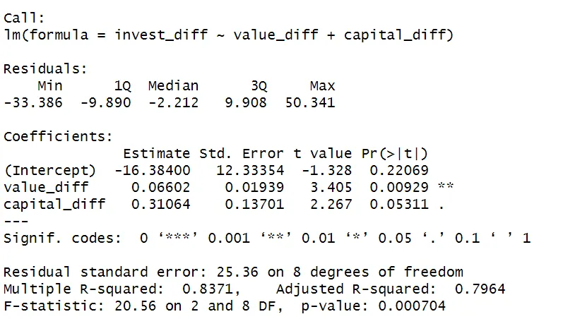
To eliminate the firm-specific characteristics $\alpha_{i}$, we can use a differencing approach. By regressing the difference in the Investment variable between 1940 and 1935 on the difference in the independent variables during that period, we arrive at the differenced regression equation:

\(invest_{i1940} - invest_{i1935} = \beta_1 (value_{i1940} - value_{i1935}) + \beta_2 (capital_{i1940} - capital_{i1935}) + (u_{i1940} - u_{i1935})\)

By taking differences between the years, we remove any unobserved variable that is constant over time: $\alpha_{i}$ is removed from the equation!

The following code block estimates this regression in R.

Entity fixed effects (panel data; $T \ge 2$ years)

Now, we will consider a fixed effects regression, by using the full Grunfeld data set ($T = 20$). With only entity fixed effects, this is the model:

\(invest_{it} = \beta_0 + \beta_1 value_{it} + \beta_2 capital_{it} + \alpha_i + \epsilon_{it}\)

where,

• $invest_{it}$ is the gross investment of firm i in year t
• $value_{it}$ is the market value of assets of firm i in year t
• $capital_{it}$ is the stock value of plant and equipment of firm i in year t
• $\alpha_i$ is the fixed effect for firm i
• $\epsilon_{it}$ is the error term, which includes all other unobserved factors that affect investment but are not accounted for by the independent variables or the fixed effects.

Entity & Time fixed effects

In this step, time fixed effects are added to the model. Time fixed effects capture the unobserved year-specific factors that are common to all firms in that year. With both time and entity fixed effects, this is the model:

\(invest_{it} = \beta_0 + \beta_1 value_{it} + \beta_2 capital_{it} + \alpha_i + \delta_t + \epsilon_{it}\)

where,

• $\alpha_i$ is the fixed effect for firm i
• $\delta_t$ is the fixed effect for year t

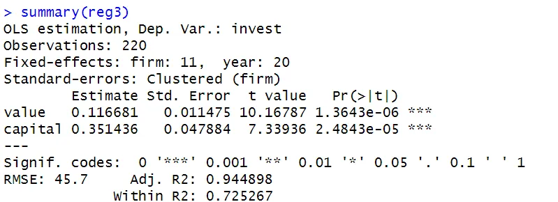
The following code estimates this fixed effects equation in R. Please refer to the fixest article for a thorough explanation on this fixed effects regression in R and the package fixest in general.