Overview

The fixest package is a powerful and versatile tool for analysing panel data in R. It is fast, memory-efficient, and offers a wide range of options for controlling the estimation process. Its main strength is the ability to estimate fixed effects models, which are commonly used in panel data analysis to control for unobserved heterogeneity at the individual or group level. Compared to others, the main advantage of the fixest package is computational prowess, which lets it estimate models in a fraction of the time compared to many other packages. This is especially consequential when your model entails highly dimensional fixed effects, i.e., fixed effects with many different levels, such as a fixed effect for several thousand stores in your sample. The “trick” fixest uses to do this is described in great detail in Bergné (2018). In addition to fixed effects models, the fixest package includes functions for estimating other (non-)linear models such as Poisson models, and negative binomial models.

Using a stylised example, we illustrate how you can use various functions in the fixest package for fixed-effect estimation. For illustration purposes, we will use the Grunfeld dataset which contains investment data for 11 U.S. Firms. It contains information on the following variables:

Variables	Description
invest	Gross investment in 1947 dollars
value	Market value as of Dec 31 in 1947 dollars
capital	Stock of plant and equipment in 1947 dollars
firm	- General Motors - US Steel - General Electric - Chrysler - Atlantic Refining - IBM - Union Oil - Westinghouse - Goodyear - Diamond Match - American Steel
year	1935-1954

Load packages

Estimation with feols()

We can estimate a fixed-effects model using the feols() function, which can be used to estimate linear fixed-effects models. The estimation equation in this example is as follows:

\(invest_{it} = \beta_0 + \beta_1 value_{it} + \beta_2 capital_{it} + \alpha_i + \delta_t + \epsilon_{it}\)

where,

• $invest_{it}$ is the gross investment of firm i in year t
• $value_{it}$ is the market value of assets of firm i in year t
• $capital_{it}$ is the stock value of plant and equipment of firm i in year t
• $\alpha_i$ is the fixed effect for firm i (capturing unobserved firm-specific factors that don’t vary over time)
• $\delta_t$ is the fixed effect for year t (capturing unobserved year-specific factors that are common to all firms in that year)
• $\epsilon_{it}$ is the error term, which includes all other unobserved factors that affect investment but are not accounted for by the independent variables or the fixed effects.

Standard Errors

When dealing with panel data, one must expect biased standard errors. An excellent paper on this issue and a good starting point for deciding how this may affect your research is Petersen (2009). Most commonly, the bias results from either correlation between different time periods of a group (a group effect) or a correlation across different groups within the same time period (a time effect). While the former is often called serial correlation, the latter is called cross-sectional dependence. For both, clustering your standard errors can be a remedy. As a free “bonus,” clustering your standard errors also helps you to address heteroskedasticity, the fact that the error term is not distributed equally across your observations.

One-way clustering is used when clustering is along one dimension only, and two-way clustering is used when clustering is along two dimensions. Usually, your clusters are either the group, the time, or both. While one-way and two-way clustering is the most commonly used ways of clustering, the number of potential clusters is not limited to two. For example, if you are a large national retailer and want to analyze customer purchases in your stores over several months, you could easily justify clustering on (1) the individual store (the group), the individual month (the time), and (3) the store’s city. By clustering your standard errors on the city, you acknowledge that some unobserved regional factors may influence stores in the same city equally. When deciding on your approach to clustering, you should also remember that clustering is only sensible when the number of clusters you create is sufficiently high. As usual with statistics, what is sufficient is subject to debate, but frequently a number between 30-50 comes up. Following that argument, if you have stores from less than 30 cities in your data, you should abstain from clustering on the city level. In addition, when you only have one store in each city, clustering on the city becomes equal to clustering on the store.

After deciding on the right way to cluster, we can cluster standard errors using the cluster option in feols() for one-way or two-way clustering.

Additionally, the vcov() function in the fixest package is a handy way to easily adjust standard errors. It returns the estimated variance-covariance matrix of the model parameters. It contains the se option which can be used to specify the type of standard errors to compute. The following standard error types can be specified:

• standard: This is the default option when no clustering is used. It computes the standard erors assuming independent and identically distributed errors. This is appropriate when the errors are uncorrelated.

• hetero: This option computes heteroskedasticity-robust standard errors. It assumed that the errors are uncorrelated but may have different variances. This is appropriate when the varianve of the errors varies across observations.

• cluster: This option computes cluster-robust standard errors. It accounts for correlation of errors within clusters. This is appropriate when there are groups of observations that are likely to be correlated with each other.

• twoway: This option computes two-way cluster-robust standard errors. It accounts for correlation of errors within two clusters, which can be useful when there are multiple sources of correlation in the data. Similarly, you can also compute threeway and fourway cluster robust standard errors using the options threeway and fourway respectively.

Export results

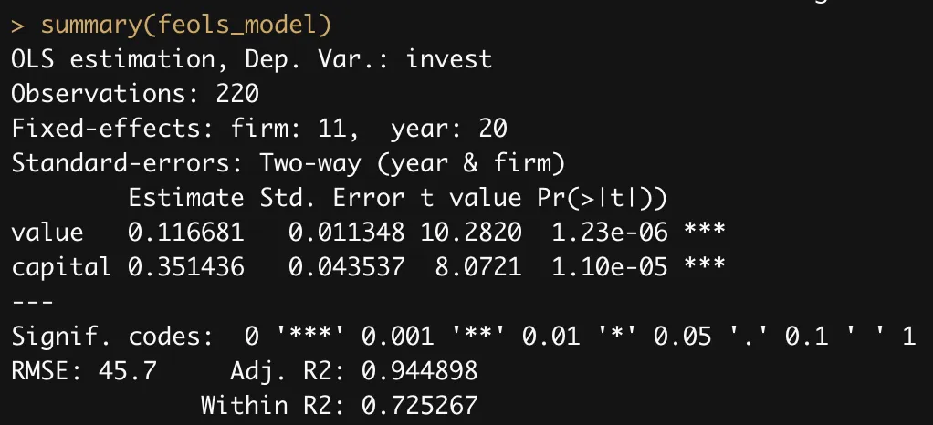
We can print a summary of the model using the summary function. Alternatively, one could also use the etable function and export the results to Latex by passing an additional argument: tex = TRUE.

Importantly, we can explicitly specify the variance-covariance matrix to be used. Continuing with our example, we had computed heteroskedasticity-robust-standard errors with two-way clustering. We can include this using the .vcov option in the summary() function and the se option under the etable() function.

Extract the fixed-effect coefficients

Use the fixef() function to obtain the fixed-effects of the estimation. The summary() method helps to get a quick overview:

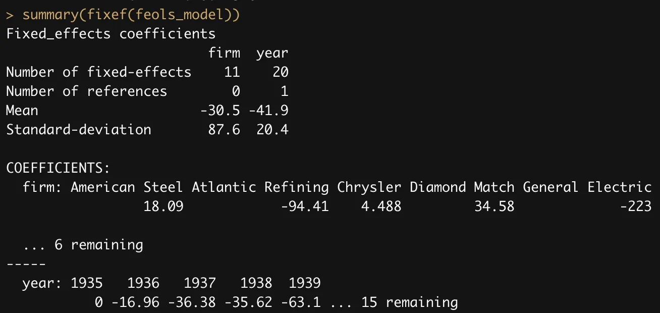
Note that the mean values are meaningless per se, but give a reference point to which to compare the fixed-effects within a dimension

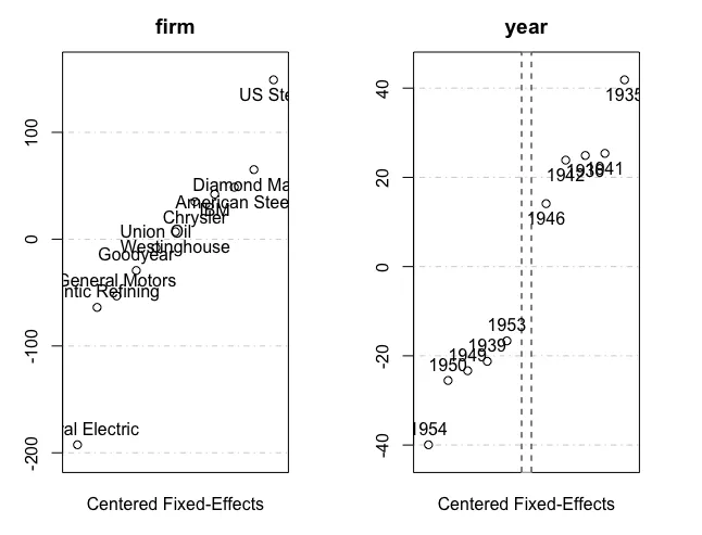
Finally, the plot function helps to distinguish the most notable fixed-effects with the highest and lowest values for each of the fixed-effect dimensions.

Other Estimation Methods in fixest

Aside from feols(), here are additional functions useful for estimation based on the model requirements:

Function	Description	Use
feglm	Generalized linear models	This function estimates fixed-effects generalized linear models, which can handle non-linear outcome variables and non-normal error distributions.
femlm	Maximum likelihood estimation	This function estimates fixed-effects maximum likelihood models, which can handle a wide range of distributions and can include both continuous and categorical variables.
feNmlm	Non-linear in RHS parameters	This function estimates fixed-effects non-linear models where the non-linearity is in the right-hand side parameters.
fepois	Poisson fixed-effect	This function estimates fixed-effects Poisson models, which are commonly used for count data that follow a Poisson distribution.
fenegbin	Negative binomial fixed-effect	This function estimates fixed-effects negative binomial models, which are commonly used for count data that exhibit over dispersion relative to the Poisson distribution.