Overview

The Pooled OLS model can only be used under the assumption of independence across groups and no error term correlation over time with the independent variables. This assumption is violated in the presence of unobserved entity-specific effects, leading to omitted variable bias. This bias arises when relevant independent variables are excluded from the regression. Hence, it is crucial to control for these unobserved effects to obtain reliable estimates.

The first-difference (FD) estimator is the first method we discuss to control for fixed effects and address the problem of omitted variables. By taking the first-difference within each cross-section, it eliminates the firm-specific effects that remain constant over time. Examples of unobserved entity-specific fixed effects in our model include factors like managerial quality, level of risk aversion, or technological advancements within firms.

Tip

Practical application of FD estimator

The Fixed Effects (FE) model discussed in the next topic is often the preferred choice in practice to address the problem of omitted variables. The FD estimator can be seen as a technical intermediary step between the Pooled OLS and the FE model.

First-difference estimator

The objective of the FD estimator is to eliminate firm-specific effects that do no vary over time, denoted by the variable $\alpha_{i}$. This is achieved by taking the first-difference of the variables within each cross-section.

The original model with fixed effects $\alpha_i$ is represented as:
\(Y_{it} = \beta_1 X_{it} + \alpha_i + u_{it}, i = 1,...,n, t = 1,...,T,\)

The first-difference transformation is applied as follows:
\(Y_{i,t} - Y_{i,t-1} = \beta_1 (X_{i,t} - X_{i, t-1}) + (\alpha_i - \alpha_i) + (u_{i,t} - u{i,t-1})\)

Since $\alpha_{i}$ is constant over time, taking the difference between consecutive years eliminates the fixed effects. This difference is represented as $\alpha_{i}$ - $\alpha_{i}$, resulting in zero.

Assumption of Error term correlation

Assumption 1 of the Fixed Effects Regression Assumptions states that the error term is uncorrelated with the independent variables, expressed as $E[u_{it}|X_{i1},…,X_{it}] = 0$.

In the context of the FD estimator, the assumption of error term correlation can be expressed in a slightly weaker form. Instead of requiring zero correlation between the error term and the independent variables at each point in time, it only requires that the difference in the error term between time $t$ and $t-1$ is uncorrelated with the difference in the independent variables between those two time periods. This weaker form is denoted as $E[u_{i,t} - u_{i,t-1}|X_{i,t} - X_{i,t-1}] = 0$.

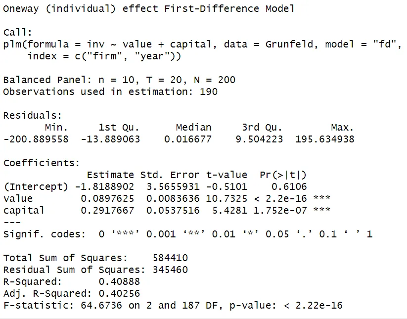
First-difference estimation in R

Similar to the pooled OLS model, the plm function can be used to estimate the FD model in R. To specify the model type as first-difference, add model = "fd".

# Load packages & data
library(plm)
library(AER) 
data(Grunfeld) 

# Estimate First-difference model
model_fd <- plm(inv ~ value + capital, 
              data = Grunfeld, 
              index = c("firm", "year"), 
              model = "fd")

summary(model_fd)

Summary

The first-difference (FD) estimator is a useful approach to address the issue of omitted variable bias in the presence of unobserved entity-specific effects. By taking the first difference within each cross-section, the FD estimator eliminates the fixed effects.

It relies on the assumption of no correlation between the difference in the error term and the difference in the independent variables over time. This is a weaker assumption than the general Fixed Effects Assumption 1. This can be seen as an advantage of the FD estimator over a Fixed Effects model. The next topic will discuss this Fixed Effects model (the Within Estimator).