


Overview
Regression models can sometimes suffer from problems such as confounding variables, measurement error, omitted variable bias (spuriousness), simultaneity, and reverse causality. This is mainly caused when the error term is correlated with the independent variable(s) and so the corresponding coefficient is estimated inconsistently, posing a threat to the internal validity of the model.
A general way of obtaining consistent estimates and solving this issue is by introducing instrumental variables in the model.
In this building block we will walk you through the process of using instrumental variables in your regression by introducing the ivreg() function from the AER package and also discuss which variables are considered to be valid instruments.
We analyse data from the mroz data set which is an in-built data set in R, provided by the wooldridge package. We are interested in examining how the education level of employees relates to their wages. Our simple regression model will be as follows:
$wage_{i} = \beta_{0} + \beta_{1} educ_{i} + \mu$
where,
| Variable | Description |
|---|---|
wage | earnings per hour |
educ | years of schooling |
Loading the data

install.packages("wooldridge")
install.packages("AER")
library(wooldridge)
library(AER)
data(mroz)
Estimating the simple regression model
Our regression model can be estimated using the following code:
lm(data=mroz, wage~educ)
This model likely suffers from endogeneity due to omitted variable bias. An employee's innate ability is likely correlated to their wages and to the level of education they have attained. As a result, the OLS estimate of the effect of education and wages is an inconsistent estimate because this variable is omitted from the model.
A possible solution is to use fatheduc as an instrument for educ. This is because a parent's level of education can serve as a proxy for the resources and opportunities available to their child. Parents with higher education often have better income, stability, and access to educational resources. Consequently, they can provide their children with a better education, which, in turn, can increase their earning potential. It is also important to note that a parent's education does not directly influence the wages their child may receive, nor does it have any direct impact on other variables that could potentially affect wages, such as the child's innate ability.
Hence, intuitively fatheduc could be a good candidate for a IV but let us check if it indeed fulfills these criterion.
Instrument validity
A valid instrument, Z is the one that fulfills the following 2 conditions:
1) Relevance: It is correlated with the independent variable, X i.e. it is relevant.
2) Exogeneity: It is not correlated with the error term, $\mu$ i.e. it is exogenous.
In other words, Z should affect the outcome variable, Y, only through X to be considered as a valid instrument.
The second condition about Instrument exogeneity cannot be tested and needs to be justified from theory or common sense.
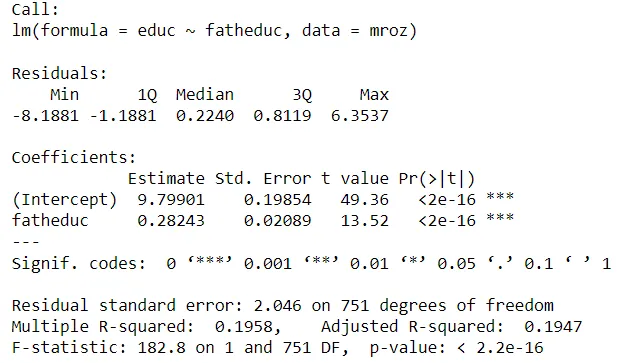
But to check if the first condition holds, we can analyse a simple regression between the instrument and the independent variable of choice.
For our model we can see below that fatheduc is indeed significantly correlated with educ and hence satisfies the condition for instrument relevance.
reg <- lm(data=mroz, educ~fatheduc)
summary(reg)
Therefore, including fatheduc as an instrument variable in a 2-Stage Least Squares (2SLS) analysis of the relationship between wage and educ can address the endogeneity issue and produce unbiased and consistent estimates.
The 2SLS estimator
The 2SLS proceeds in the following way:
In the first stage, the variation in the endogenous independent variable, X is decomposed into a problem-free component that is explained by the instrument, Z and a problematic component that is correlated with the error,$\mu_{i}$
$educ_{i} = \gamma_{0} + \gamma_{1} fatheduc_{i} + \epsilon_{i}$
where $\gamma_{0}$ + $ \gamma_{1}fatheduc_{i} $ is the component of $educ_{i}$ that is explained by $fatheduc_{i}$ while $\epsilon_{i}$ is the component that cannot be explained and exhibits correlation with $\mu$
In the second stage, the problem-free component of the variation in X is used to estimate $\beta_{1}$
$wage_{i} = \beta_{0} + \beta_{1} \hat{educ_{i}} + \mu$
Estimating the regression using ivreg()
To run the instrumental variable regression, we use the ivreg() function which is offered by the AER package. It works similar to the lm() function but includes an additional argument for the instrument, separated from the regression equation by a vertical line, |.
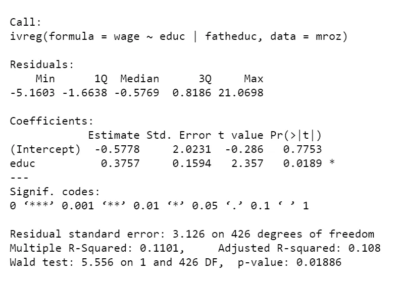
iv <- ivreg(data=mroz, wage~educ|fatheduc)
summary(iv)
Test for instrument strength
Although fatheduc is a valid instrument, it could still not be a very strong one. This could be because it is not that significantly correlated with the independent variable.
To check the strength of the instrument in your model, you can use the diagnostics = TRUE argument in the summary() function as follows:
summary(iv, diagnostics = TRUE)
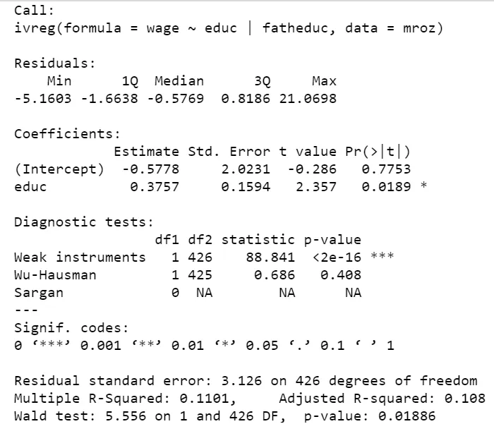
This gives you information about 3 tests:
1)Weak instrument:
A good instrumental variable is highly correlated with one or more of the explanatory variables while remaining uncorrelated with the errors. If an endogenous regressor is only weakly related to the instrumental variables, then its coefficient will be estimated imprecisely. We hope for a large test statistic and small p-value in the diagnostic test to significantly say that our instrument is strong, as is the case in our example.
2)Wu-Hausman:
Applied to 2SLS regression, the Wu–Hausman test is a test of endogeneity. If all of the regressors are exogenous, then both the OLS and 2SLS estimators are consistent, and the OLS estimator is more efficient, but if one or more regressors are endogenous, then the OLS estimator is inconsistent. Again, we need a large test statistic and a small p-value for the OLS estimator to be inconsistent. However, it is not true in our example and the 2SLS estimator is therefore not to be preferred.
3)Sargan:
The Sargan test is a test of overidentification. That is, in an overidentified regression equation, where there are more instrumental variables than coefficients to estimate it is possible that the instrumental variables provide conflicting information about the values of the coefficients. Unlike in the other 2 tests, a large test statistic and small p-value for the Sargan test suggest that the instruments are not valid. In our case, we obtain NA values for this test as we have an equal number of instrumental variables and coefficients.
 Summary
-
Instrument variables address the issue of endogeneity and help obtain consistent estimates.
-
For an instrument to be valid, it should be
relevantandexogenous. It should affect the outcome variable, Y only through the independent variable, X. -
The
iv_reg()function from theAERpackage can be used to run an instrumental variable regression in R. -
The strength of the instrument can be tested via 3 tests: Weak instrument test, Wu-Hausman test and Sargan test. These can be obtained using the
diagnostics = TRUEargument in thesummary()function.