Overview

The parallel trends assumption, introduced in the Intro to Difference-in-Difference topic, is crucial for establishing causality in a DiD design. However, this assumption may not always hold.

A common approach to test whether this assumption holds is testing the difference in pre-treatment trends. However, this method knows some limitations. Here, we cover an alternative approach of Rambachan & Roth (2019), which handles violations of the parallel trends assumption, introducing the HonestDiD package in R.

Tip

Reasons for an invalid parallel trends assumption

The parallel trends assumption can be violated in various scenarios. For example:

1. Different pre-treatment trends: Pre-treatment trends differ for treatment and control groups.

2. Hidden trends: Non-parallel trends can exist even with similar pre-trends. Non-linear trends may hide an underlying difference, especially with a short pre-treatment period.

3. Low statistical power: The statistical power is too low to detect violations of parallel trends, even if they are present.

4. Economic shock: A shock occurs around the treatment period, causing differences in post-treatment trends, even if the pre-treatment trends were similar.

Rejecting the hypothesis of pre-trends does not confirm that the trends are similar. Always justify the parallel trends assumption within your research context, rather than relying solely on test outcomes suggesting similar pre-trends!

The HonestDiD approach

Rambachan & Roth (2019) propose a method to address potential violations of the parallel trends assumptions by relaxing this assumption.

The framework

Instead of relying on zero pre-treatment differences in trends, an alternative is to extrapolate the existing difference to the post-treatment period. This approach identifies the causal effect by assuming the post-treatment difference in trends is precisely similar to the pre-treatment difference. This strong assumption is often unrealistic.

Rambachan & Roth's framework modifies this idea by allowing for an interval of differences in trends, based on the pre-existing difference. They recognize that while the post-treatment difference in trends between the treated and control groups often may not be exactly the same as the pre-treatment difference, it is similar to some degree.

Summary

The key idea is to restrict the possible values of the post-treatment difference to a certain interval based on the known pre-trend difference.

This method results in partial identification, estimating an interval rather than a precise coefficient.

How to choose these restrictions?

Selecting the right restrictions on how much the pre and post-treatment trends can differ depends on your study's specifics, including the economic context and potential confounding factors. Here are two approaches to guide these choices and to formalize the restrictions:

1. Relative magnitude bounds

If you believe the confounding factors causing deviations from parallel trends after treatment are similar in size to those before treatment, the Relative magnitude bounds approach is suitable. This method uses the pre-treatment to set limits on the post-treatment trend differences, helping us account for any violations. Specifically, parameter $\bar{M}$ sets bounds on the size of the post-treatment violations based on observed pre-treatment violations. For example, setting $\bar{M}$ to 1 assumes post-treatment violations are, at most, the same size as pre-treatment violations, while $\bar{M}$ = 2 allows the post-treatment violations to be up to twice the size of the pre-treatment violations.

Example

Benzarti and Carloni (2019) estimated the effect of a value-added tax decrease on restaurant profits in France. They were concerned about unobserved macroeconomic shocks affecting restaurants (treatment group) differently than other service sectors (control group), leading to a violation of the parallel trends assumption. However, it is reasonable to assume that the trend differences after the tax change are not much larger than those before the tax change, motivating the use of the Relative Magnitude bounds approach in this context.

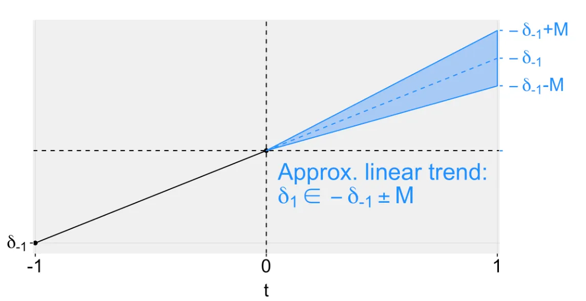
1. Smoothness restriction

When you expect the differences in trends between the treatment and control group to evolve smoothly over time without sharp changes, the Smoothness restriction approach is appropriate. This method assumes that the post-treatment violations will not deviate much from a linear extrapolation of the pre-trend violations while allowing for some flexibility (M > 0) to account for deviations from a perfect linear trend.

Example

Lovenheim and Willén (2019) studied the impact of a specific law on adult labor market outcomes of the affected students. They compared people across states and birth cohorts, leveraging the different timings of the law's implementation. Their main concern was the presence of long-term trends that might differ systematically with treatment, such as changes in labor supply or educational attainment. These trends likely evolve smoothly over time, making the smoothness restriction approach suitable.

Tip

Additional possible restrictions

• Combination of Smoothness and Relative Magnitude bounds

If you believe that trends change smoothly over time, but are unsure about the exact level of smoothness (M ≥ 0), you can combine the smoothness and relative magnitude bounds approaches to set reasonable limits on trend changes. This method assumes that any non-linear changes after the treatment are limited by the non-linear changes observed before treatment.

• Sign and monotonicity

If you expect the bias to consistently go in a particular direction (either always positive or always negative), you can include this as a restriction as well.

Non-staggered DiD example

We continue with the Goodreads example introduced in the DiD regression topic. Here, we examine the effect of a newly introduced Q&A feature on subsequent book ratings, using Goodreads as the treatment group and Amazon as the control group. We have 2 groups (Amazon vs Goodreads) and 2 time periods (pre and post-Q&A).

The baseline analysis relies on the parallel trend assumption. If we are concerned about the validity of this assumption, we can conduct a sensitivity analysis using the HonestDiD package. This package incorporates the approach introduced earlier, allowing for a more flexible examination of the parallel trends assumption.

Tip

The full code for this example is available in this Gist.

Follow these steps to conduct the sensitivity analysis in the non-staggered example analysis:

1. Load the necessary packages and clean the data

See the Gist for the code.

1. Install the HonestDiD package

You can install and load the HonestDiD package running the following code:

• R

# Make it possible to install from GitHub 
install.packages("remotes") 

# Don't allow for warning errors stopping the installation
Sys.setenv("R_REMOTES_NO_ERRORS_FROM_WARNINGS" = "true")

# Install HonestDiD package from GitHub
remotes::install_github("asheshrambachan/HonestDiD")

1. Estimate the baseline model

The resulting coefficients and covariance matrix are saved under betahat and sigma:

• R

# Run model
model_4 <- feols(rating ~ i(goodr, qa) | year_month + asin,
                cluster = c("asin"),
                data = GoodAma)

# Save coefficients
betahat <- summary(model_4)$coefficients

# Save the covariance matrix
sigma <- summary(model_4)$cov.scaled

1. Estimate DiD with Relative Magnitude bounds

• R

delta_rm_results <- createSensitivityResults_relativeMagnitudes(
    betahat = betahat, #coefficients
    sigma = sigma, #covariance matrix
    numPrePeriods = 1, #num. of pre-treatment coefs
    numPostPeriods = 1, #num. of post-treatment coefs
    Mbarvec = seq(0.5,2,by=0.5) #values of Mbar
  )

delta_rm_results

Output:

R
# A tibble: 4 × 5
     lb     ub method Delta    Mbar
          
1 -6.74 -2.57  C-LF   DeltaRM   0.5
2 -6.74 -0.344 C-LF   DeltaRM   1  
3 -6.74  2.41  C-LF   DeltaRM   1.5
4 -6.74  5.18  C-LF   DeltaRM   2

The results show that if Mbar is set at 0.5 or 1 (assuming the post-Q&A trend violation is at most as large as the pre-Q&A trend violation), a negative effect of the Q&A feature on book ratings is found, as the confidence interval (from lower bound lb to upper bound ub) includes only negative values. However, when Mbar is set larger than 1, the interval includes zero, indicating no evidence of a causal impact.

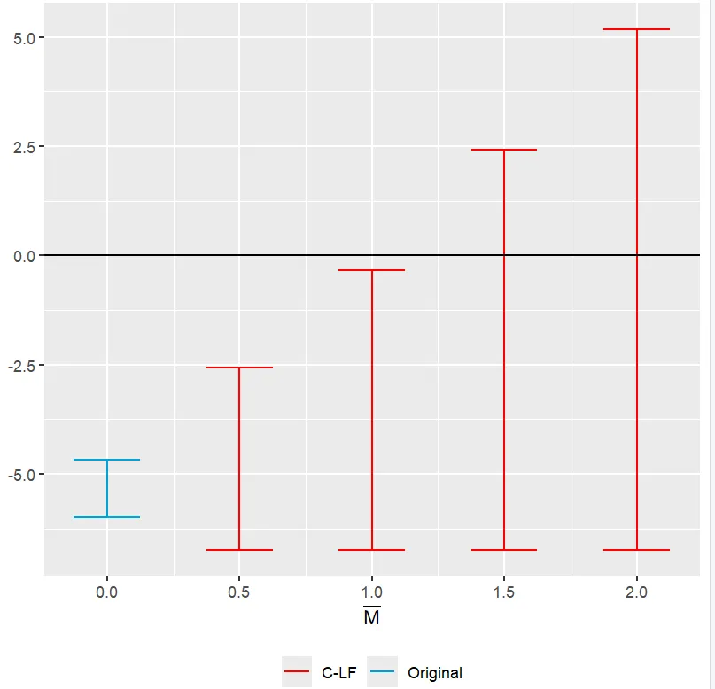
1. Create a plot

The plot compares the baseline results with the results of the RM approach, showing the threshold to find an impact is Mbar = 1.

• R

plot_rm <- HonestDiD::createSensitivityPlot_relativeMagnitudes(delta_rm_results, originalResults)
plot_rm

Staggered DiD example

This example demonstrates how to use the HonestDiD approach with a staggered DiD framework, continuing the staggered Goodreads example.

Tip

The full R code for this example is shared in this GitHub Gist.

Follow these steps to conduct a staggered DiD sensitivity analysis:

1. Specify the function

To combine the staggered DiD approach of Callaway and Sant'Anna (using the did package) and the HonestDiD package, a function is created by Sant'Anna as the packages are not fully integrated yet. Extract the function from the HonestDiD GitHub page, or from the Gist created for this example.

1. Load packages and data

Run the code in the Gist to load the necessary packages and get the dataset ready to use for analysis.

1. DiD estimation

With the honest_did specified in Step 1, and the dataset goodreads_df loaded in Step 2, use the following for the sensitivity analyses and plots:

• R

# 3.1. Staggered DiD analysis 

staggered_results <- did::att_gt(yname = "rating", # outcome var
                          tname = "period_review", # time var
                          idname = "asin", # individual var
                          gname = "period_question", # treated
                          control_group = "notyettreated", #control
                          data = goodreads_df, # final dataset
                          allow_unbalanced_panel = TRUE,
                          base_period = "universal")

# Aggregate results 
es <- did::aggte(cs_results, type = "dynamic", na.rm = TRUE)


# 3.2 SENSITIVITY ANALYSIS: RELATIVE MAGNITUDES 

sensitivity_results_rm <-
  honest_did(es,
             e=0,
             type="relative_magnitude",
             Mbarvec=seq(from = 0.5, to = 2, by = 0.5))

HonestDiD::createSensitivityPlot_relativeMagnitudes(sensitivity_results_rm$robust_ci,
                                                    sensitivity_results_rm$orig_ci)


# 3.3 SENSITIVITY ANALYSIS: SMOOTHNESS RESTRICTIONS

sensitivity_results_sd <-
  honest_did(es = es,
             e = 0,
             type="smoothness")


HonestDiD::createSensitivityPlot(sensitivity_results_sd$robust_ci,
                                sensitivity_results_sd$orig_ci)

The following plots are generated:

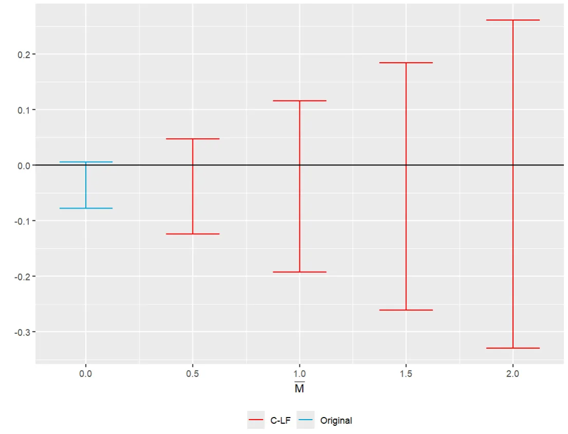
1. Relative magnitudes

1. Smoothness restriction

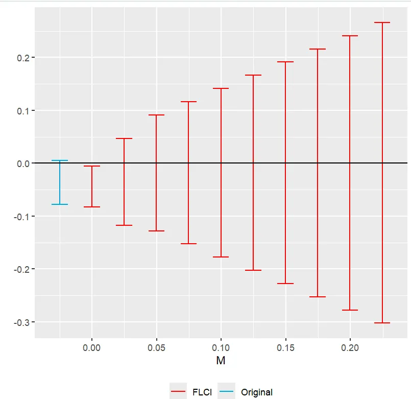
The Relative Magnitudes and Smoothness Restrictions graphs show confidence intervals that include zero for each value of M. Thus, no evidence of a causal effect is found in the staggered case under the assumptions made.

Summary

The HonestDiD approach by Rambachan & Roth (2019) addresses violations of the parallel trends assumption in DiD analysis by extrapolating pre-treatment differences to the post-treatment period and allowing for an interval of differences. This method can serve as a sensitivity analysis, enhancing the credibility of causal inference in DiD studies!

While the assumptions about the relationship between post- and pre-trend differences are very context-specific, there are two main approaches to setting restrictions and specifying your framework (with possible combinations of these approaches):

1. Relative magnitude bounds: Sets limits based on pre-treatment differences.
2. Smoothness restriction: Assumes trends evolve smoothly over time.

References

• Rambachan and Ruth (2019) - A More Credible Approach to Parallel Trends

• GitHub Page HonestDiD, Example Application

• Blog post of David Mckenzie: What happens if the parallel trends assumption is (might be) violated?