


Overview
While randomized controlled experiments are considered the gold standard for establishing causality, they aren't always practical, feasible, or ethically permissible. In such cases, quasi-experimental methods offer a valuable alternative, using natural variations in treatment or exposure to approximate controlled experimental conditions.
 Tip
TipYou can find an introduction to causal inference here.
Difference-in-Differences (DiD) is one such quasi-experimental method commonly used to evaluate the causal impact of a treatment or intervention. The DiD framework is used in a wide range of settings, from evaluating the impact of a rise in the minimum wage to assessing how the adoption of online streaming affects music consumption and discovery.
 Summary
DiD estimates the treatment effect by comparing changes in outcomes between a treatment and control group before and after the treatment is implemented. In other words, it examines the difference in the difference between these groups.
Setup
Suppose we are studying the effectiveness of a new educational program (the treatment) on students' test scores. The treatment group consists of students who received the program ($D_i = 1$), and the control group of students who did not receive the program ($D_i = 0$). The setup table for DiD is:
| Before (\$Y_i^0\$) | After (\$Y_i^1\$) | |||
|---|---|---|---|---|
| Control (\$D_i = 0\$) | \$E(Y_i^0\ | D_i = 0)\$ | \$E(Y_i^1\ | D_i = 0)\$ |
| Treatment (\$D_i=1\$) | \$E(Y_i^0\ | D_i = 1)\$ | \$E(Y_i^1\ | D_i = 1)\$ |
Some outcomes are counterfactual, representing what would have happened if treatment statuses were reversed. Naturally, an individual cannot simultaneously be treated and not treated. Therefore, we only observe one of the two potential outcomes for each person after treatment implementation: the treated outcome for those who received treatment and the untreated outcome for those who did not.
One might think of simply taking the difference in the average outcome before and after for the treatment group ($Y_1^0-Y_1^1$). However, this approach fails because the treatment occurrence and time are perfectly correlated, making it impossible to isolate the treatment effect from the temporal effects. Similarly, comparing the average outcomes of the treated and control groups in the after period ($Y_1^1-Y_0^1$) is problematic because natural differences between the groups may confound results. The group receiving the program is for example on average more motivated independent of receiving the treatment.
To address these issues, double differencing (difference-in-difference) is done, which involves taking differences between the outcomes of the control group from those of the treatment group before and after treatment to estimate the treatment effect.
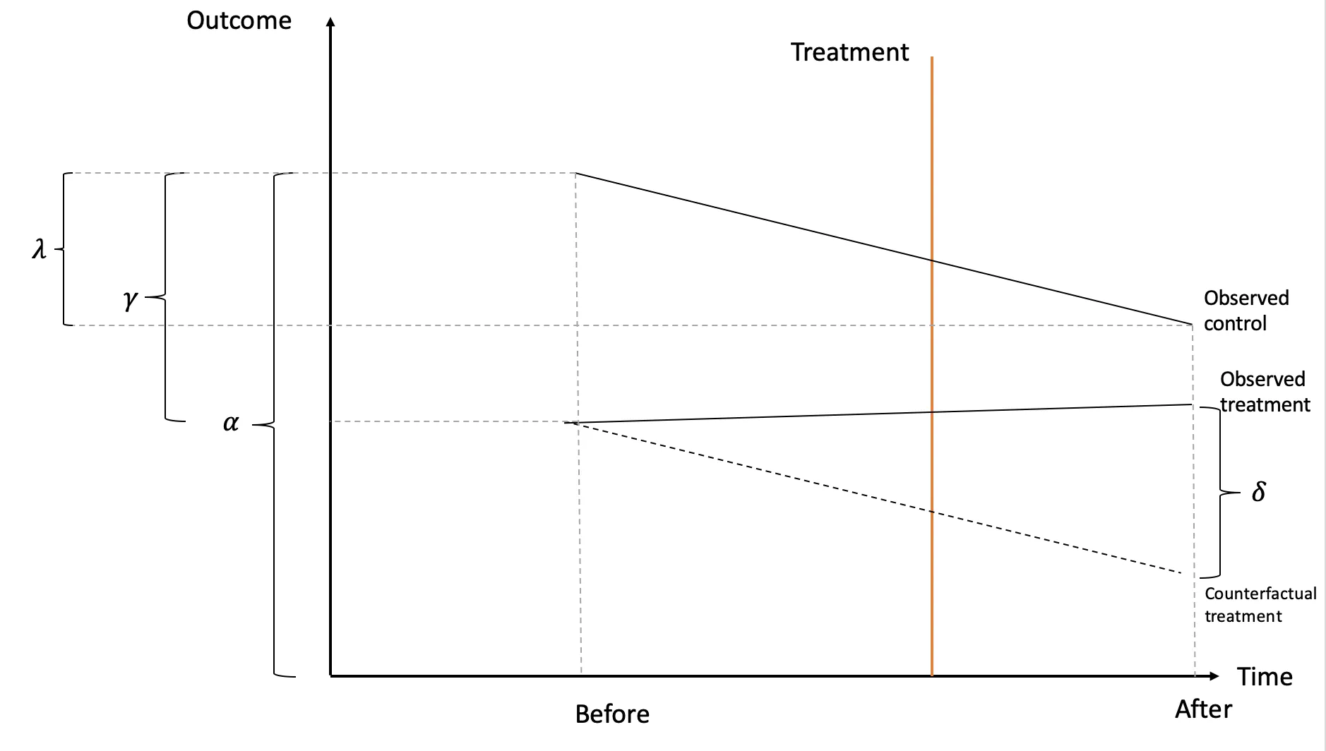
| Before | After | After - Before | |
|---|---|---|---|
| Control | $\alpha$ | $\alpha + \lambda$ | |
| Treatment | $\alpha + \gamma$ | $\alpha+\gamma+\lambda+\delta$ | |
| Treatment - Control | $\gamma$ | $\gamma+\delta$ | $\delta$ |
By taking the difference between the treatment and control groups’ outcomes before treatment ($\gamma$) and the difference between their outcomes after treatment ($\gamma + \delta$), we can obtain the final treatment effect ($\delta$), which is the additional change in outcome for the treatment group compared to the control group after the treatment is implemented.
Tip$\gamma$ represents any differences in outcomes between the treatment and control groups, that exist before the treatment is implemented. $\lambda$ represents the common change in outcomes over time that affects both the treatment and control groups equally.
Identifying assumptions
To establish causality using the DiD design, two key assumptions are necessary:
- Parallel Trends Assumption
In the absence of treatment, the treatment and control groups would have followed similar trends over time. It ensures that any differences in outcomes observed before the treatment between the two groups are due to pre-existing differences, as the trends are assumed to be parallel.
More formally, it assumes that the difference between the control group's counterfactual outcome ($E(Y_i^1|D_i = 0)$) and its observed outcome before treatment ($E(Y_i^0|D_i = 0)$) would remain constant over time. Similarly, it assumes that the difference between the treatment group's observed outcome after treatment ($E(Y_i^1|D_i = 1)$) and its counterfactual outcome ($E(Y_i^0|D_i = 1)$) would also remain constant over time.
- Conditional Independence (Unconfoundedness) Assumption
Conditional on observed variables, the treatment assignment is independent of potential outcomes.
This ensures that there are no confounding factors that simultaneously affect both the treatment assignment and the potential outcomes. After controlling for observable covariates, the treatment assignment is then random with respect to potential outcomes.
Now that we have covered all the basics, let's jump to an example to put all this theory into practice!
Example: The 2x2 DiD Table
On May 21, 2014, Goodreads, a social cataloging website for books, introduced the Q&A feature, enabling users to post questions to authors and fellow readers. It is intriguing to explore the potential impact of this feature on subsequent book ratings. For example, users now have the opportunity to proactively inquire about a book before making a purchase. This interaction may help alleviate uncertainties regarding the book's suitability, potentially reducing customer dissatisfaction and mitigating the likelihood of negative reviews.
The dataset used in this example includes information on book ratings and their corresponding dates from both Goodreads and Amazon. In this analysis, we will treat the implementation date of the Q&A policy as the treatment and assess its impact on subsequent book ratings through the employment of the DiD approach. As Amazon lacks the Q&A feature specifically for the book category but still permits consumers to rate and review books akin to Goodreads, it serves as a suitable control group for comparison. You can find the complete data preparation and analysis code in this Gist to follow along.
Since we have 2 groups (Amazon Vs Goodreads) and 2 time periods (pre-Q&A and post-Q&A), we use the canonical 2 x 2 DiD design.

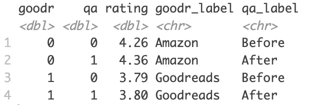
# Compute the average rating for the treatment and control group, before and after the Q&A launch
means<- GoodAma %>%
  group_by(goodr, qa) %>%
  summarize(rating=mean(rating)) %>%
  ungroup()

# Modify the labels
means_modified <- means %>%
  mutate(
    goodr_label = case_when(
      goodr == 0 ~ "Amazon",
      goodr == 1 ~ "Goodreads"
    ),
    qa_label = case_when(
      qa == 0 ~ "Before",
      qa == 1 ~ "After"
    )
  )
print(means_modified)
Here, we compute the average rating for the treatment and control group both before and after the Q&A launch based on the GoodAma dataframe. The treatment dummy, goodr = 1 indicates the treatment group (Goodreads), and otherwise the control group (Amazon). The time dummy, qa = 1 indicates the after period and 0 for the before period.
Now, let’s compute the treatment effect by double differencing.
# before-after for untreated, has time effect only

bef_aft_untreated <- filter(means, goodr == 0, qa == 1)$rating - filter(means, goodr == 0, qa == 0)$rating

# before-after for treated, has time and treatment effect
bef_aft_treated<- filter(means, goodr == 1, qa == 1)$rating - filter(means, goodr == 1, qa == 0)$rating

# difference-in-difference: take time +treatment effect, and remove the time effect
did<- bef_aft_treated - bef_aft_untreated

print(paste("Diff in Diff Estimate: " , did))
The obtained results indicate that the presence of the Q&A feature is associated with lower ratings. Note that the differences-in-means table is merely suggestive and should be interpreted with caution. To obtain more accurate and reliable estimates, it is essential to conduct a regression analysis, which allows to control for variables and examine the statistical significance of the results. Refer to the next topic to continue with this example as a DiD regression!
SummaryDifference-in-Difference (DiD) is a powerful statistical method for evaluating the causal impact of a treatment or intervention. It compares changes in outcomes between a treatment group and a control group before and after the treatment is implemented. Assumptions crucial for a causal interpretation of the estimates are the parallel trends assumption and the conditional independence assumption.
An example is given to illustrate how to obtain the difference-in-means table for a 2x2 DiD design. To learn how to estimate the effect with regression analysis, refer to the next topic.